NCL Home>
Application examples>
Plot techniques ||
Data files for some examples
Example pages containing:
tips |
resources |
functions/procedures
NCL Graphics: Plotting data on a map using gsn_csm_xxx functions
This page is an introduction to using
the
gsn_csm_xxxx_map
functions to plot data (contours, vectors, streamlines) over a map.
All of the data files for the examples below can either be found on the
data page, or via instructions
included in the scripts.
KNOW YOUR DATA
To correctly plot data on a map, you must KNOW YOUR DATA.
What type of latitude (lat) / longitude (lon) structure
is your data on?
- Rectilinear grid
- Curvilinear grid
- Random points
- Unstructured mesh
To determine what kind of lat/lon structure your data is on, use a
UNIX command line tool
like ncl_filedump on
your data file, or use printVarSummary after you
read a data variable. The examples below explain how to identify your
lat/lon structure.
Is your data global or regional?
If your data is regional (i.e. it doesn't cover the full map), then
you may need to:
- Set the special gsnAddCyclic resource to False.
- Set additional map resources to zoom in on the map area of interest.
Do your lat/lon arrays have units of "degrees_north" and "degrees_east"?
If your lat/lon arrays don't have "units" attributes, or they don't
have "degrees" type of units, then your data may not plot correctly.
See
example 7 below for how to fix this.
Is your data large?
If you have a big grid or mesh that you want to generate
contours for, then you may want to do "raster fill"
contours instead of "area fill" contours for faster plotting.
See examples 8 and 13.
Does your data need to be reordered to be plotted correctly?
If your data variable is a two-dimensional (2D) array ordered lon x
lat, you will need to reorder it to be lat x
lon. See example 8 below.
Is your lat/lon data not in degrees?
If your lat/lon data is in radians or meters or some units other than
"degrees" you will need to convert it to degrees before you can plot
your data. See example 13 below.
Is your data already projected onto a particular map projection?
If your data is already projected onto a particular map projection,
this is called data on a
native grid.
If you know the exact parameters for the map
projection, then you can plot the data without needing any lat / lon
arrays at all. This can significantly speed up plotting because the
data doesn't need to go through a mathematical transformation to be
plotted correctly.
To plot data in its native projection, you first have to set up the
map projection parameters EXACTLY as what your data are projected
onto, and then set
res@tfDoNDCOverlay to True (or the
equivalent "NDCViewport", in NCL V6.5.0)
It is possible to plot data on a native grid in a different map
projection, if you have the lat/lon values for each data
point. However, if you do this, you do NOT want to
set tfDoNDCOverlay to True, because
now you are not plotting in a native projection.
For examples of plotting data both in a native projection and a different
projection, see examples 3,
4, and 10 below.
Is your data "packed" on the file?
Sometimes data is "packed" on a file to save space. This means you
will need to unpack it before it will plot correctly. If your data is
of type "short" or "byte" when you read it off the file, then this may
be a indication that you need to unpack it. See
example 9 below.
Does the data itself have errors?
If you have everything correct in your script and the data still is
not being plotted correctly, then some possible sources of the problem
can be:
- Not having the correct units for your lat/lon arrays
- Having NaN values in your data
- Having data that needs to be "unpacked"
- Not having the correct missing value (_FillValue attribute)
If you do have problems, LOOK AT YOUR DATA:
- Use printVarSummary and
printMinMax to look
at your data, your lat/lon arrays, and
your metadata.
- Pay close attention to any warnings or errors
that are produced when running your script.
For examples of fixing "bad" data, see examples 7
and 12 below.

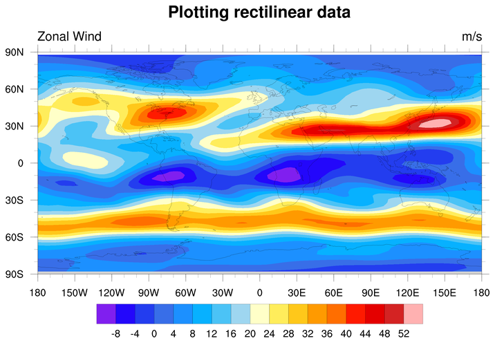
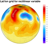
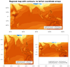
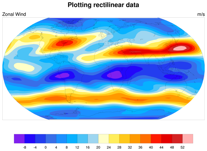
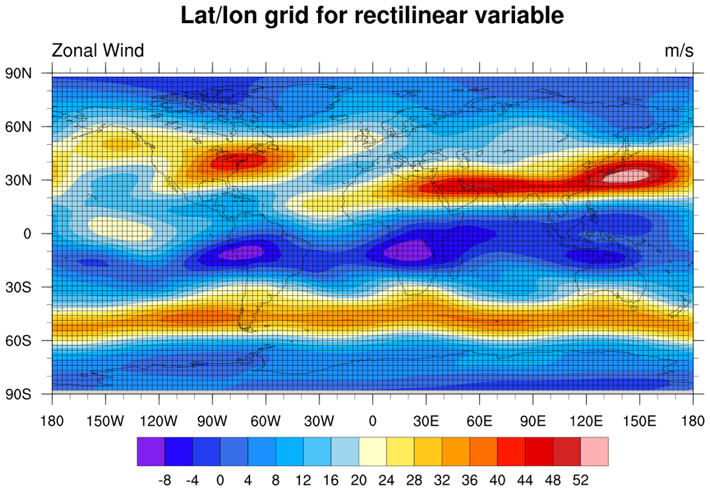
 dataonmap_1.ncl
 /
dataonmap_grid_1.ncl
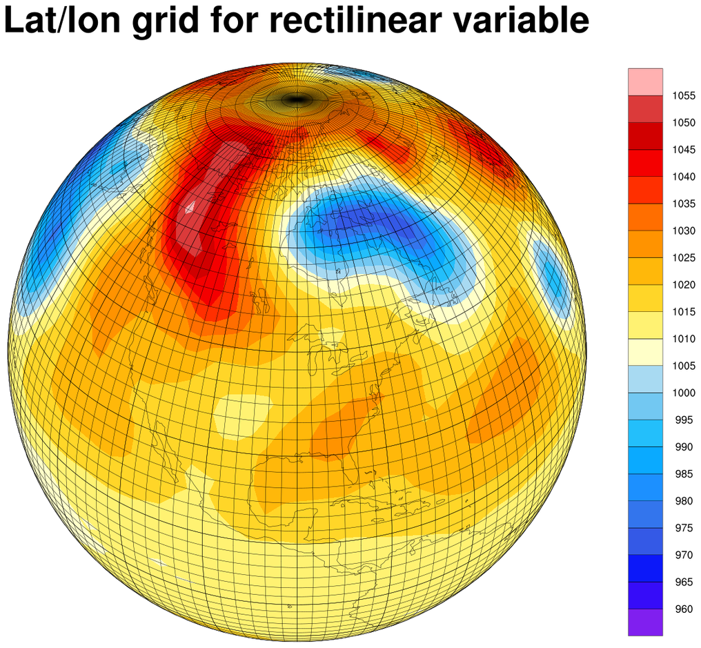
Rectilinear grid
Data: uv300.nc (NetCDF file, included
with NCL distribution)
Data on a rectilinear grid
is the simplest data to plot because the latitude and longitude
coordinate arrays are automatically attached to the data variable when
you read it in.
You can quickly tell if your data is on a rectilinear grid
by looking at the printVarSummary output
of your data variable:
   Variable: u
   Type: float
   Total Size: 32768 bytes
               8192 values
   Number of Dimensions: 2
   Dimensions and sizes : [lat | 64] x [lon | 128]
   Coordinates :
            lat : [-87.8638..87.8638]
            lon : [-180..177.1875]
   Number Of Attributes : 5
   time : 1
   _FillValue : -999
   long_name : Zonal Wind
   units : m/s
Note the "Coordinates:" line, which is followed by two lines
indicating the range of the "lat" and "lon" arrays. This means you
have data on a rectilinear grid. If your data is on any other type of
grid (curvilinear, unstructured mesh, random), then there will
be no lat/lon arrays listed after the "Coordinates:" line.
To plot this data, simply read the "u" variable and pass it to
gsn_csm_contour_map. This
function will look for coordinate arrays attached to "u", and will
use them for plotting:
  u = a->U(0,:,:)

  wks = gsn_open_wks("png","dataonmap")

  res              = True
  res@cnFillOn     = True
  res@tiMainString = "Plotting rectilinear data"

  plot = gsn_csm_contour_map(wks,u,res)
The second frame shows how easy it is to plot the data on a different
map projection, simply by setting
mpProjection to the desired
projection, like "Robinson".
The third frame is from the
dataonmap_grid_1.ncl
script. It demonstrates how to call
gsn_coordinates to add the
lat/lon lines associated with your data.
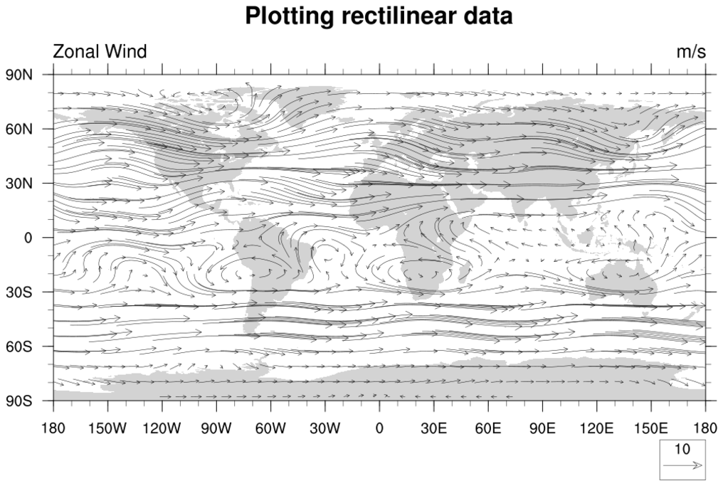
 dataonmap_2.ncl
Rectilinear grid
dataonmap_2.ncl
Rectilinear grid
Data: uv300.nc (NetCDF file, included
with NCL distribution)
This is the same rectilinear grid as the previous example, except a
vector plot is drawn. Both "u" and "v" have coordinate arrays attached
to them, so there's nothing special you need to do to correctly plot this
over a map.
   Variable : u
   Type : float
   . . .
   Number of Dimensions: 2
   Dimensions and sizes: [lat | 64] x [lon | 128]
   Coordinates:
               lat: [-87.8638..87.8638]
               lon: [-180..177.1875]
   Number Of Attributes: 5
    . . .

   Variable: v
   Type: float
   . . .
   Number of Dimensions: 2
   Dimensions and sizes: [lat | 64] x [lon | 128]
   Coordinates:
               lat: [-87.8638..87.8638]
               lon: [-180..177.1875]
   Number Of Attributes:  5
   . . .
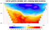
 dataonmap_3.ncl
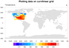
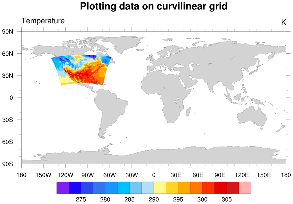
Curvilinear grid
dataonmap_3.ncl
Curvilinear grid
Data: ruc.grb (GRIB file)
Data on a curvilinear grid
is data whose latitude / longitude coordinates are represented by
2-dimensional (2D) latitude / longitude arrays.
When you read a data variable represented by 2D lat/lon arrays, these
arrays will NOT be attached as coordinate arrays to the data like they
are with rectilinear data.
First, note the output from printVarSummary. It
has a "Coordinates" line, but there are no coordinate variables listed
after it:
    Variable: temp
    Type: float
    Number of Dimensions: 3
    Dimensions and sizes: [lv_SPDY3 | 6] x [gridx_236 | 113] x [gridy_236 | 151]
    Coordinates:
    Number Of Attributes: 13
    . . .
This means you don't have any lat/lon data attached to this
variable, and hence this data is not rectilinear.
Second, note that there is a "coordinates" attribute attached
to your variable with the string value "gridlat_236 gridlon_236":
    Variable: temp
    . . .
    Number Of Attributes: 13
    long_name : Temperature
    units : K
    _FillValue : 1e+20
    coordinates : gridlat_236 gridlon_236
    . . .
If you do have a "coordinates" attribute, then it most likely
includes the names of the variables on the file that contain that
variable's lat/lon coordinate information, in this case "gridlat_236"
and "gridlon_236".
Doing a "ncl_filedump" on this file indeed shows these two variables
exist on the file, and they are both 2-dimensional and the same size
as the lat/lon dimensions of the data variable. This means you have
data on a curvilinear grid.
   Variable: gridlat_236 (file variable)
   Type: float
   . . .
   Number of Dimensions: 2
   Dimensions and sizes: [gridx_236 | 113] x [gridy_236 | 151]
   Coordinates:
   Number Of Attributes: 15
   . . .

   Variable: gridlon_236 (file variable)
   Type: float
   . . .
   Number of Dimensions: 2
   Dimensions and sizes: [gridx_236 | 113] x [gridy_236 | 151]
   Coordinates:
   Number Of Attributes: 15
  . . .
To plot data on a curvilinear grid, you must read these 2D lat/lon
variables from the file and attach them to the data variable as special
attributes called "lat2d" and "lon2d":
  . . .
  temp       = a->TMP_236_SPDY   ; 6 x 113 x 151
  temp@lat2d = a->gridlat_236    ;     113 x 151
  temp@lon2d = a->gridlon_236    ;     113 x 151
  . . .
  res          = True
  res@cnFillOn = True

  plot = gsn_csm_contour_map(wks,temp(0,:,:),res)
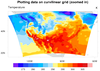
In the second frame of this example, we simply zoom in on the area of
interest, by setting the mpMinLatF
/ mpMaxLatF
/ mpMinLonF
/ mpMaxLonF resources.
The third frame is from
the dataonmap_grid_3.ncl
script. It demonstrates how to
call gsn_coordinates to add the
lat/lon lines associated with your data.
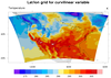
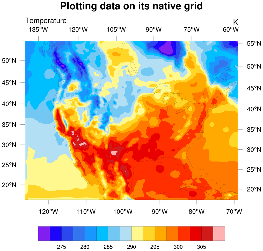
 dataonmap_native_3.ncl
 /
dataonmap_native_grid_3.ncl
Curvilinear grid in a native projection
Data: ruc.grb (GRIB file)
This script plots the same data as the previous example, except
it plots the data on its native grid
using map projection information attached as attributes to the
lat/lon arrays on the file:
  a    = addfile("ruc.grb","r")
  lat  = a->gridlat_236      ; Needed only for projection information
  lon  = a->gridlon_236
  . . .
  res@mpLeftCornerLatF  = lat@corners(0)
  res@mpLeftCornerLonF  = lon@corners(0)
  res@mpRightCornerLatF = lat@corners(2)
  res@mpRightCornerLonF = lon@corners(2)

  res@mpProjection        = lat@mpProjection
  res@mpLambertMeridianF  = lat@mpLambertMeridianF
  res@mpLambertParallel1F = lat@mpLambertParallel1F
  res@mpLambertParallel2F = lat@mpLambertParallel2F
When plotting data natively, you must set the
special
tfDoNDCOverlay resource to
True (or the equivalent "NDCViewport", in NCL V6.5.0), to tell NCL not
to do a map transformation.
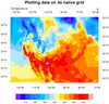
The second frame is from
the dataonmap_native_grid_3.ncl
script. It demonstrates how to
call gsn_coordinates to add the
lat/lon lines associated with your data.
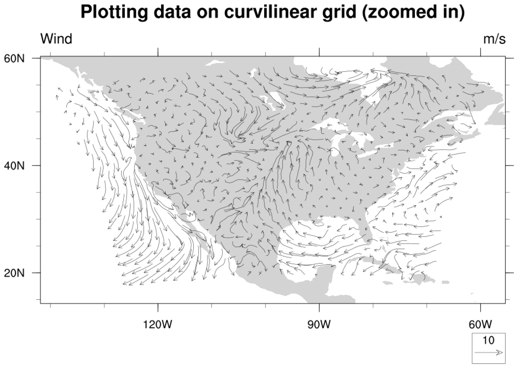
 dataonmap_4.ncl
Curvilinear grid
dataonmap_4.ncl
Curvilinear grid
Data: ruc2.bgrb.20020418.i12.f00 (GRIB file)
This GRIB file is similar to the previous one, in that
the data variables contain a "coordinates" attribute
indicating the name of the lat/lon variables on the file.
This time a vector plot is being drawn. The special "lat2d" /
"lon2d" arrays must be attached to both the u and v data
arrays.
  u       = f->U_GRD_252_HTGL
  v       = f->V_GRD_252_HTGL
  lat2d   = f->gridlat_252
  lon2d   = f->gridlon_252
  u@lat2d = lat2d
  u@lon2d = lon2d
  v@lat2d = lat2d
  v@lon2d = lon2d
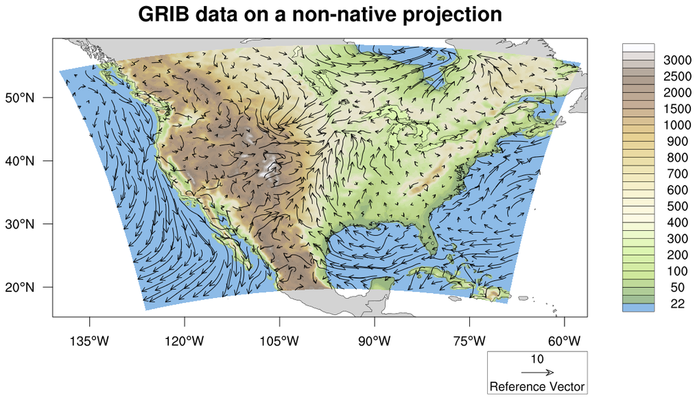
 dataonmap_native_4.ncl
 /
dataonmap_nonnative_4.ncl
Curvilinear grid plotted in both native and non-native projections
Data: ruc2.bgrb.20020418.i12.f00 (GRIB file)
The "native" script plots the same curvilinear vector data as in the
previous example, except using the Lambert Conformal native map
projection parameters provided on the file. It also overlays the
vectors on filled geopotential height contours, which are on the same
lat/lon curvilinear grid.
As with example dataonmap_native_3.ncl, the
map projection information is obtained from special attributes
attached to the lat/lon arrays, and the special
resource tfDoNDCOverlay is set to
True.
The "nonnative" version of the script plots the exact same data in a basic
cylindrical equidistant map projection.
 dataonmap_5.ncl
 /
dataonmap_5_640.ncl /
dataonmap_grid_5.ncl
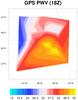
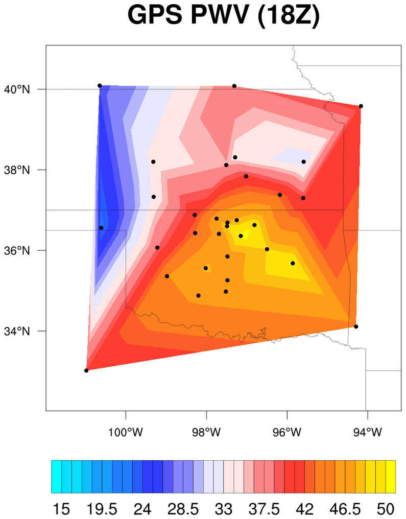
Random data
Data: pw.dat (ASCII file)
If you have a one-dimensional (1D) array of data represented by 1D
lat/lon arrays of the same length, then this is considered to either
be an "unstructured mesh" or "random points".
This example shows how to plot 32 random data points, given a lat/lon
value for each point. The data are read off
the ASCII file using asciiread.
To correctly plot random data over a map, you must set the
special sfXArray
and sfYArray resources to the
one-dimensional longitude / latitude arrays, respectively:
  pwv = tofloat(str_get_field(lines(1:),4," "))
  lat = tofloat(str_get_field(lines(1:),2," "))
  lon = tofloat(str_get_field(lines(1:),3," "))
  . . .
  res          = True
  res@cnFillOn = True
  res@sfXArray = lon
  res@sfYArray = lat

  plot = gsn_csm_contour_map(wks,pwv,res)
NCL will internally interpolate the data to a triangular mesh before
plotting it.
You cannot currently plot vectors that are on random points or an
unstructured mesh.
In NCL Version 6.4.0, you will be able to use special "lat1d" and
"lon1d" attributes to plot the data
(see dataonmap_5_640.ncl). There's
no real advantage to this method over the sfXArray / sfYArray method,
except that it's similar to the model for curvilinear data that uses
the "lat2d" and "lon2d" attributes:
  pwv       = tofloat(str_get_field(lines(1:),4," "))
  pwv@lat1d = tofloat(str_get_field(lines(1:),2," "))
  pwv@lon1d = tofloat(str_get_field(lines(1:),3," "))
  . . .
  res          = True
  res@cnFillOn = True

  plot = gsn_csm_contour_map(wks,pwv,res)
The second frame shows how to plot the 32 random lat/lon locations
using gsn_coordinates.
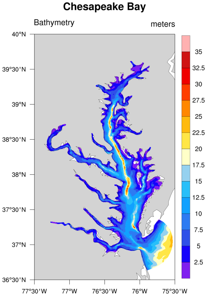
 dataonmap_6.ncl
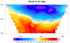
Triangular mesh
dataonmap_6.ncl
Triangular mesh
Data: ctcbay.nc (NetCDF file, included
with NCL distribution)
If you have 1D data and lat/lon arrays all the same length, and you
also have a variable that contains a triangular mesh of your data, then
you can set the
special sfElementNodes resource
to this connectivity mesh for faster plotting results:
  . . .
  x   = f->data     ; 1D array of data (length npts)
  lat = f->lat      ; 1D array of data (length npts)
  lon = f->lon      ; 1D array of data (length npts)
  ele = f->ele      ; n x 3 (triangular mesh that connects the cells)
  . . .
  res                = True
  res@sfYArray       = lat
  res@sfXArray       = lon
  res@sfElementNodes = ele
  res@cnFillOn       = True
  . . .
  plot = gsn_csm_contour_map(wks,depth,res)
Note that the leftmost dimension of the triangular mesh will likely be
larger than the length of your 1D data arrays.
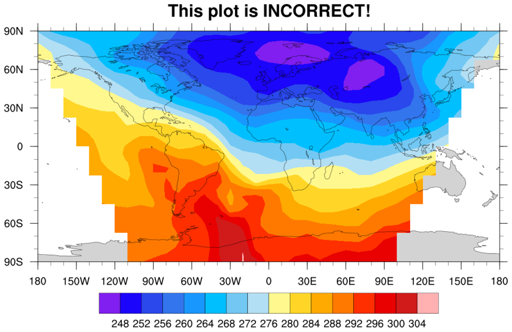
 dataonmap_7.ncl
 /
dataonmap_grid_7.ncl
Rectilinear grid
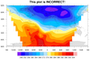
Data: Tstorm.cdf (NetCDF file, included with NCL distribution)
The data for this example is on a rectilinear grid, but if you
try to plot it the usual way, you will get the following warnings
and an incorrect plot:
  check_for_y_lat_coord: Warning: Data either does not contain a valid
  latitude coordinate array or doesn't contain one at all.
  A valid latitude coordinate array should have a 'units'
  attribute equal to one of the following values:
  'degrees_north' 'degrees-north' 'degree_north' 'degrees north'
This is due to the fact that the lat/lon arrays do not have "units"
attributes of "degrees_north" and "degrees_east" respectively:
   Variable: lat (coordinate)
   . . .
   Number of Dimensions: 1
   Dimensions and sizes: [lat | 33]
   Coordinates:
   Number Of Attributes: 0

   Variable: lon (coordinate)
   . . .
   Number of Dimensions: 1
   Dimensions and sizes: [lon | 36]
   Coordinates:
   Number Of Attributes: 0
You can fix this by attaching the expected "units" attribute to both coordinate
arrays, via the "t" data variable:
   t&lat@units = "degrees_north"
   t&lon@units = "degrees_east"
You will then get a second error:
   gsn_add_cyclic: Warning: The range of your longitude data is not 360.
   You may want to set the gsnAddCyclic resource to False to avoid a
   warning message from the spline function.
This can be fixed by setting the special gsnAddCyclic to
resource to False as suggested.
The second frame shows the result of the plot once you add the missing
"units" and turn off the cyclic point. The third frame simply zooms
in on the map area of interest.
The last frame is from
the dataonmap_grid_7.ncl
script. It demonstrates how to
call gsn_coordinates to add markers
at lat/lon locations associated with your data. The red markers
indicate areas where the data contains missing values.
 dataonmap_8.ncl
Rectilinear grid
dataonmap_8.ncl
Rectilinear grid
Data: 3B-MO.MS.MRG.3IMERG.20140701-S000000-E235959.07.V03D.HDF5 (HDF5 file)
The data for this example is on a rectilinear grid, but it is ordered
longitude x latitude:
   Variable: p
   Type: float
   . . .
   Number of Dimensions: 2
   Dimensions and sizes: [lon | 3600] x [lat | 1800]
   Coordinates:
               lon: [-179.95..179.95]
               lat: [-89.95..89.95]
   Number Of Attributes: 6
   . . .
In order to plot this data correctly, it must
be reordered to be lat
x lon. In this script, the reordering is done right inside the
plotting call, but you could also do it earlier in the script,
like when reading in the variable.
plot = gsn_csm_contour_map(wks, p(lat|:,lon|:), res)
This is a rather large grid (3600 x 1800). In order to speed up the
plotting, we are using "raster" fill for the contours
(cnFillMode="RasterFill"). This
can make things SIGNIFICANTLY faster for large grids.
The default contour fill mode is "AreaFill". If you try to contour
this data using "AreaFill", you will get a fatal error:
ContourPlotDraw: Workspace reallocation would exceed maximum size 100000000
You can increase the "workspace size", but it's not really
worth it! Here are the timing results between using
"RasterFill" and "AreaFill":
  AreaFill:   Elapsed time = 1070.93 CPU seconds.
  RasterFill: Elapsed time = 1.01304 CPU seconds.
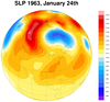
 dataonmap_9.ncl
dataonmap_grid_9.ncl
Curvilinear grid
dataonmap_9.ncl
dataonmap_grid_9.ncl
Curvilinear grid
Data: slp.1963.nc (NetCDF file)
The data for this example is "packed" on the file. That is, it is of
type "short" and you must multiply or divide it by a "scale factor" to
get the correct values. Sometimes you must also add or subtract an
"add offset" value. NCL will not do this automatically! Use functions
like short2flt
or short2flt_hdf to help you
unpack the data.
If you see data that is type "short" or "byte", this is usually an
indication that it has to be unpacked before you can do calculations
with it or plot it. You can further identify whether data needs to be
unpacked by the examining the printVarSummary
output for the presence of attributes "scale_factor" and/or
"add_offset" or something similar:
   Variable: slp
   Type: short
   Number of Dimensions: 3
   Dimensions and sizes: [time | 365] x [lat | 73] x [lon | 144]
   Coordinates:
        time: [17198568..17207304]
        lat: [90..-90]
        lon: [ 0..357.5]
   Number Of Attributes: 17
   long_name : mean Daily Sea Level Pressure
   units : Pascals
   add_offset : 119765
   scale_factor : 1
   valid_range : ( 87000, 115000 )
   actual_range : ( 94395, 111535 )
   missing_value : 32766
   _FillValue : 32766
   . . .
You should also call printMinMax
on "slp_short" to look at the min/max:
mean Daily Sea Level Pressure (Pascals) : min=-25370 max=-8230
From these min/max values, you can see right away that these are not
not valid numbers for pressure.
In this script, the short2flt
function is used to unpack the data. This function also copies over
the metadata. For a "cleaner" plot, we converted the values to "hPa"
by mutiplying by 0.01 and updated the "units" attribute to reflect
this change.
  slp_float = short2flt(slp_short)    ; unpack the data
  slp_float = slp_float * 0.01        ; convert to hPa
  slp_float@units = "hPa"             ; update the units
Calling printMinMax on
"slp_float" results in reasonable values:
mean Daily Sea Level Pressure (hPa) : min=943.95 max=1115.35
Important note about packed data:
The COARDS and CF conventions require the following formula and the
specific names "scale_factor" and "add_offset":
x = xShort*scale_factor + add_offset
Many NASA (mainly HDF) require:
x = (xShort-add_offset)*scale_factor
Since there are no specific required names,
the short2flt function looks for
many names:
  "add_offset", "offset", "OFFSET", "Offset", "_offset",
  "Intercept", "intercept", "add_off", "ADD_OFF"

  "scale", "SCALE", "Scale", "_scale", "scale_factor", "factor",
  "Scale_factor", "Slope" , "slope", "ScaleFactor", "Scale_Factor",
  "SCALING_FACTOR"
The short2flt_hdf function looks
for these names:
  "add_offset", "offset", "OFFSET", "Offset", "_offset",
  "Intercept", "intercept", "scalingIntercept", "INTERCEPT",
  "add_off"

  "scale", "SCALE", "Scale", "_scale", "scale_factor",
  "Scale_factor", "Slope" , "slope", "ScaleFactor",
  "Scale_Factor", "scalingSlope", "SCALING_FACTOR",
  "SCALE_FACTOR", "SLOPE"
Sometimes the metadata on the file will provide information on how the
data should be unpacked, or you may need to find some documentation on
your file. Generally, the "scale_factor" attribute is the value that
you multiply your data by, and the "add_offset" attribute is the value
that you add after you multiple the scale factor. If you have a
well-written file, then the metadata may also indicate a "valid range"
for your data (see above output). This makes it easier to examine your
results and make sure you are unpacking the data correctly.
The second frame is from
the dataonmap_grid_9.ncl
script. It demonstrates how to
call gsn_coordinates to add
the lat/lon lines associated with your data.
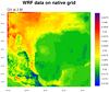
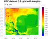 dataonmap_10.ncl
Curvilinear grid
dataonmap_10.ncl
Curvilinear grid
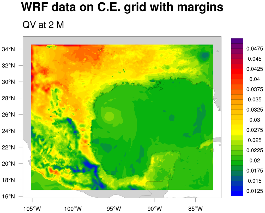
Data: wrfout_d01_2003-07-15_00:00:00 (NetCDF WRF output file)
This example plots data on a WRF-ARW grid, which is on a curvilinear
grid.
The first frame plots the data using
the native map projection on
the file. The second frame plots the data by reading the XLAT / XLONG
arrays off the file and attaching them to "q2" via the special "lat2d"
/ "lon2d" attributes.
This is an older WRF-ARW file, whose variables do not contain any
metadata that describes the lat / lon coordinates. WRF-ARW lat/lon
arrays have names like "XLAT", "XLONG", "XLAT_U", "XLONG_U", "XLAT_V",
"XLONG_V", etc. If you're not sure which ones to use, look at size of
your data variable and pick the corresponding XLAT/XLONG variable that
matches the size of your data variable.
"XLAT" and "XLONG" are used in this example, but these are the only
lat/lon arrays on this particular file.
   Variable: q2
   Type: float
   . . .
   Number of Dimensions: 3
   Dimensions and sizes: [Time | 1] x [south_north | 160] x [west_east | 180]
   Coordinates:
   Number Of Attributes: 5
   FieldType : 104
   MemoryOrder : XY
   description : QV at 2 M

   float XLAT ( Time, south_north, west_east )
   FieldType :104
   MemoryOrder :XY
   description :LATITUDE, SOUTH IS NEGATIVE
   units : degree

   float XLONG ( Time, south_north, west_east )
   FieldType : 104
   MemoryOrder : XY
   description : LONGITUDE, WEST IS NEGATIVE
   units : degree
Newer WRF ARW files will have a "coordinates" attribute for the data
variables that help you identify the correct lat/lon arrays associated
with your data. For example:
   float SST ( Time, south_north, west_east )
   FieldType : 104
   MemoryOrder : XY
   description : SEA SURFACE TEMPERATURE
   units : K
   coordinates : XLONG XLAT

   float V ( Time, bottom_top, south_north_stag, west_east )
   FieldType : 104
   MemoryOrder : XYZ
   description : y-wind component
   units : m s-1
   stagger : Y
   coordinates : XLONG_V XLAT_V
A Python version of this projection is available here.
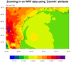
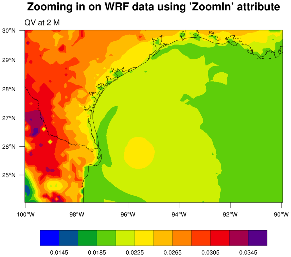
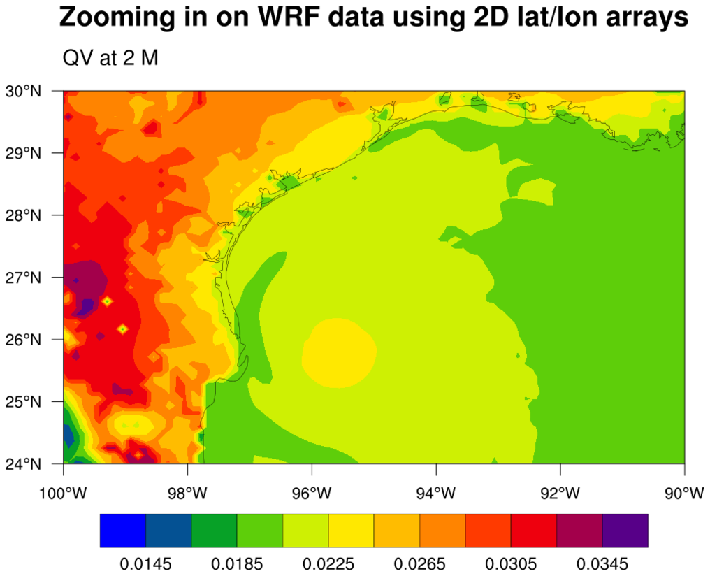
 dataonmap_zoom_10.ncl
Curvilinear grid
dataonmap_zoom_10.ncl
Curvilinear grid
Data: wrfout_d01_2003-07-15_00:00:00 (NetCDF WRF output file)
This example plots the same data as the previous example, except now we are zooming in
on a lat/lon area of interest. This example shows two ways to zoom in on WRF-ARW data:
1) using the same native WRF map projection, or 2) plotting the data in a different map
projection.
The first plot shows how to plot the data in the native map
projection by first using the
wrf_user_ll_to_xy function to
calculate the x,y index locations into the 'q2' array that represent
the approximate lat/lon area of interest. These index values are
used with the 'ZoomIn' resource to set the special Xstart, Xend, Ystart, and Yend
resources before you call
wrf_map_resources to set the
correct NEW native map projection parameters.
The second plot shows how to plot the data using the 2D lat/lon arrays
read off the file. In this case, you don't need the special index
values, because NCL will use the lat/lon arrays to figure out the
correct subset of the data to plot.
You may notice that the two plots are not plotted in the exact same
lat/lon area. This is because the lat/lon corners of the first plot
are only *approximately* equal to the requested lat/lon area of
interest. The wrf_user_ll_to_xy
function gives you the i,j indexes that are closest to the actual
lat/lon area of interest.
The second plot is the exact area requested, because NCL now has the
actual lat/lon arrays, and can use this to interpolate the data
as needed, in the area of interest.
For another example of subsetting a WRF map domain, see the
"wrf_Zoom.ncl" example
at http://www2.mmm.ucar.edu/wrf/OnLineTutorial/Graphics/NCL/Examples/SPECIAL/wrf_Zoom.htm
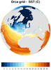
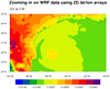
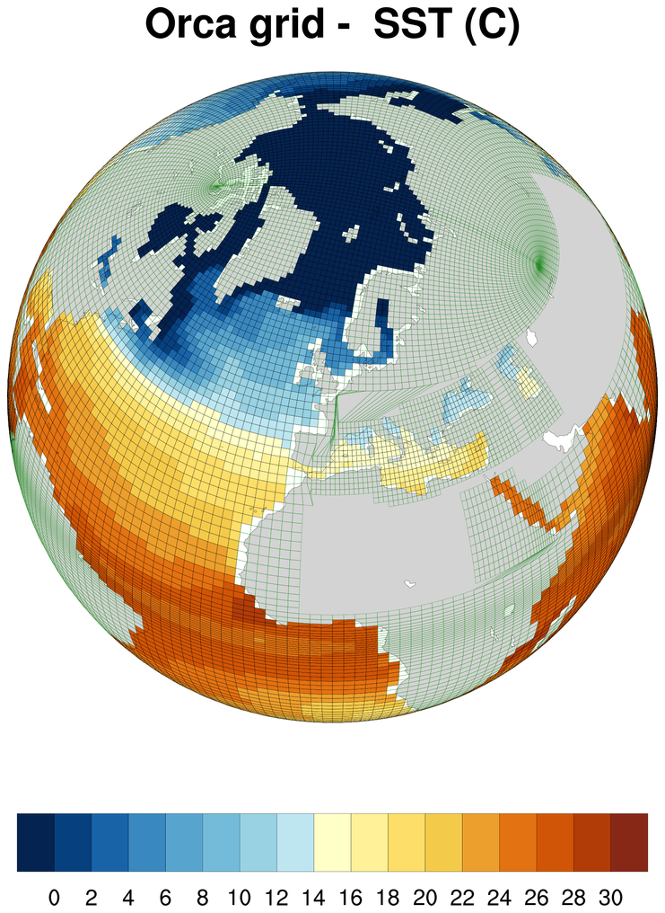
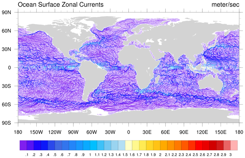
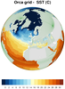 dataonmap_11.ncl
Curvilinear grid
dataonmap_11.ncl
Curvilinear grid
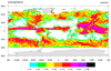
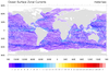
Data: ctorca.nc (NetCDF file)
This example plots data on an ORCA (ocean model) grid, which is on a
rather quirky, non-uniform curvilinear grid (see the second frame).
Note that the "sst" variable doesn't have a "coordinates" attribute,
but it does have an "associate" attribute with the string value
"time_counter nav_lat nav_lon":
   Variable: sst
   Type: float
   . . .
   Number of Dimensions: 2
   Dimensions and sizes: [y | 149] x [x | 182]
   Coordinates:
   Number Of Attributes: 13
   time_counter : 43200
   units : C
   missing_value : 1e+20
   valid_min : 1e+20
   valid_max : -1e+20
   long_name : SST
   short_name : sosstsst
   associate : time_counter nav_lat nav_lon
   _FillValue : 1e+20
Based on an educated guess, we looked for "nav_lat" and "nav_lon"
on the file, and were able to use these for the "sst"
"lat2d" / "lon2d" data attributes.
The contours are drawn in "CellFill" mode. The second frame turns on
the cell edges so you can actually see the structure of this
non-uniform grid.
 dataonmap_12.ncl
Rectilinear grid
dataonmap_12.ncl
Rectilinear grid
Data: Download any one of the NetCDF files from:
ftp://podaac-ftp.jpl.nasa.gov/OceanCirculation/oscar/preview/L4/resource/LAS/oscar_third_deg_180/
This example plots streamlines on a relatively large rectilinear
lat/lon grid (481 x 1081). Note the "NaN" ("not a number") values for
the "_FillValue" and "missing_value" attributes when you do a
printVarSummary of the data:
   Variable: u
   Type: double
   . . .
   Number of Dimensions: 4
   Dimensions and sizes:[time | 33] x [depth | 1] x [latitude | 481] x [longitude | 1081]
   Coordinates:
            time: [8488..8650.667]
            depth: [15..15]
            latitude: [  80.. -80]
            longitude: [-180.. 180]
   Number Of Attributes: 4
   units : meter/sec
   long_name : Ocean Surface Zonal Currents
   missing_value : nan
   _FillValue : nan
The NaN values are suspicious, so we also
used printMinMax to check the
min/max of the data:
   Ocean Surface Zonal Currents (meter/sec) : min=nan   max=nan
   Ocean Surface Meridional Currents (meter/sec) : min=nan   max=nan
You cannot have any NaN values in your data when plotting
with NCL, so you must use the replace_ieeenan function
to replace these values with missing values. Once you do this, the min/max
values look more reasonable:
   Ocean Surface Zonal Currents (meter/sec) : min=-3.518722   max=3.7021546
   Ocean Surface Meridional Currents (meter/sec) : min=-3.319664   max=3.662057
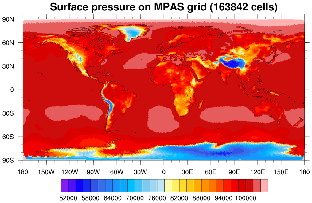
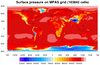 dataonmap_13.ncl
 /
dataonmap_13_640.ncl
Hexagonal mesh
Data: MPAS.nc (NetCDF file)
This example shows how to create a filled contour plot of data on a
hexagonal mesh (163,842 cells). The data and the lat/lon arrays are
all one-dimensional arrays of the same length:
   Variable: sp
   Type: double
   Number of Dimensions: 1
   Dimensions and sizes: [nCells | 163842]

   Variable: latCell
   Type: double
   Number of Dimensions: 1
   Dimensions and sizes: [nCells | 163842]

   Variable: lonCell
   Type: double
   Number of Dimensions: 1
   Dimensions and sizes: [nCells | 163842]
A couple of notes:
- The lat/lon arrays on this file are in
"radians" and must be converted to "degrees".
- Raster contours
(cnFillMode="RasterFill") are
used here for faster plotting.
As with the previous unstructured examples, you must set the
special sfXArray
and sfYArray resources to the
one-dimensional lat / lon arrays, respectively, or use the "lat1d" /
"lon1d" attributes if you have NCL V6.4.0 or later:
If you have NCL V6.3.0 or earlier:
  RAD2DEG = 180.0d/(atan(1)*4.0d)  ; Radian to Degree
  sp      = f->surface_pressure(0,:)    ; 163842 points
  lonCell = f->lonCell * RAD2DEG        ; ditto
  latCell = f->latCell * RAD2DEG        ; ditto
  . . .
  res          = True
  res@cnFillOn = True
  res@sfXArray = lonCell
  res@sfYArray = latCell

  plot = gsn_csm_contour_map(wks,x,res)
If you have NCL V6.4.0 or later:
  RAD2DEG = get_r2d("float")            ; new function in V6.4.0
  sp       = f->surface_pressure(0,:)
  sp@lat1d = f->latCell * RAD2DEG
  sp@lon1d = f->lonCell * RAD2DEG
  . . .
  res          = True
  res@cnFillOn = True
  plot = gsn_csm_contour_map(wks,sp,res)
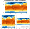
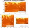
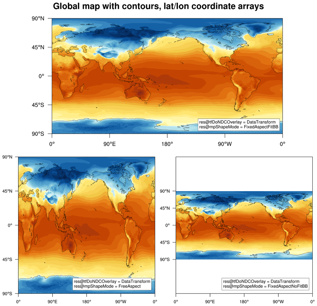
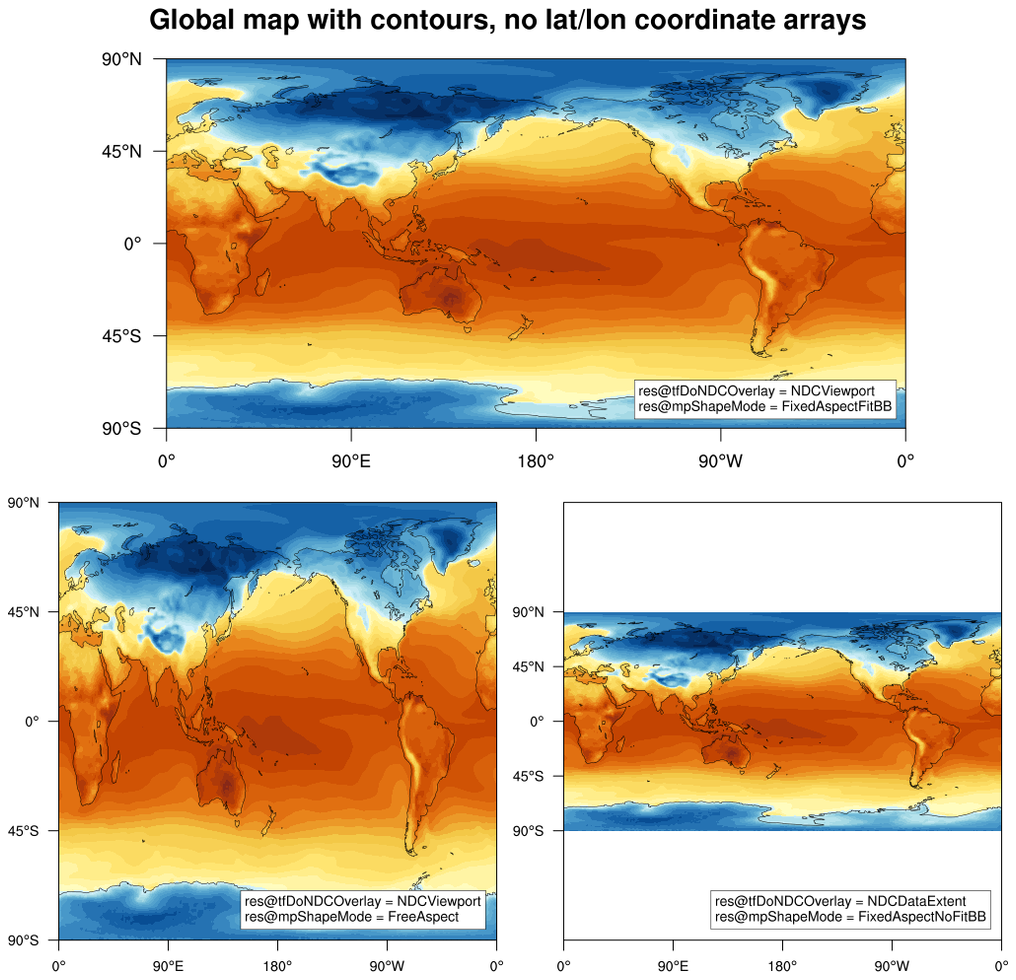
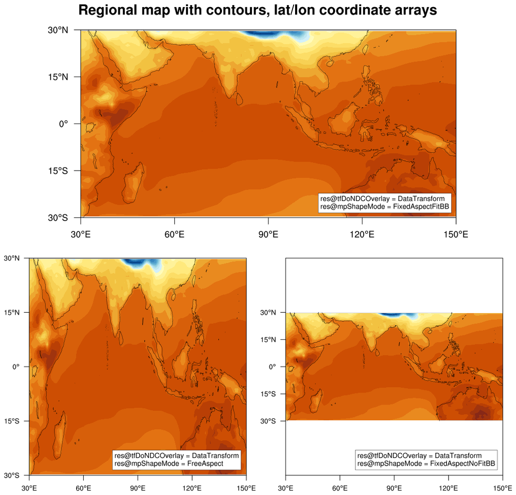
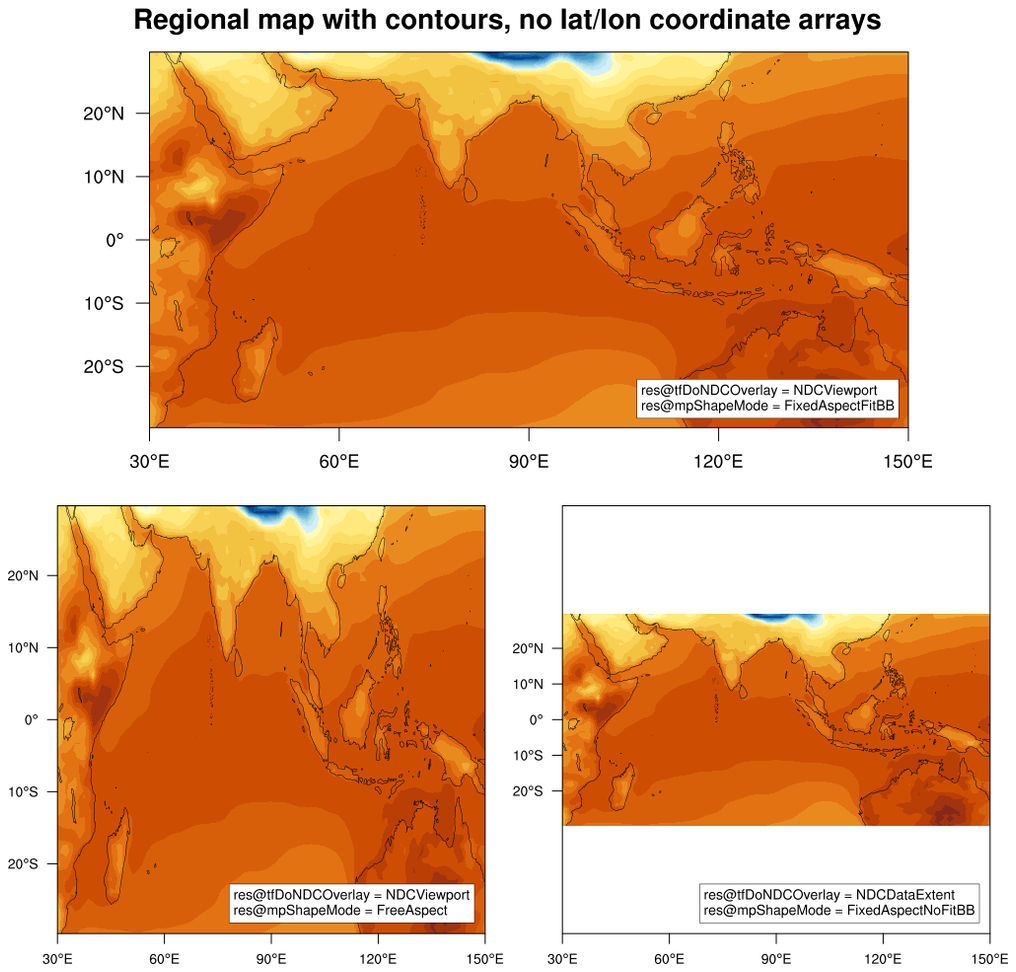
 dataonmap_14.ncl
 /
Rectilinear grid
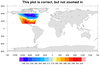
Data: ts_Amon_CESM1-CAM5_historical_r1i1p1_185001-200512.nc (NetCDF file)
The purpose of this script is to further illustrate the difference
between plotting data that contains lat/lon coordinates, and plotting
data in its native map projection (without lat/lon coordinate arrays).
In this case, we are plotting rectilinear data, so the native
projection is effectively the default projection (cylindrical
equidistant). You just have to make sure that when you plot it
natively, you give it the correct min/max lat and lon values. In this
case, the latitude values for this data go from -90 to 90, and the
longitude values go from 0 to 358.75, so all we need to set, really,
is the maximum longitude (mpMaxLonF)
to 358.75 (because NCL uses -90 to 90 and 0 to 360 by default).
Additionally, this example shows how to plot both types of data when
using the three different values
of mpShapeMode:
- FixedAspectFitBB (default)
- FreeAspect
- FixedAspectNoFitBB
The "FixedAspectNoFitBB" is not a commonly used setting, but if you do
use it and you are plotting your data natively, then you need to make
sure that
tfDoNDCOverlay is set to "NDCDataExtent".
Here are the three possible values for tfDoNDCOverlay:
- DataTransform (default)
- NDCViewport
- NDCDataExtent
The first two frames are global plots, the first frame being the
data with lat/lon coordinate arrays, and the second being
data without lat/lon coordinate arrays.
The third and fourth frames are regional plots, with the third frame being
the data with lat/lon coordinate arrays, and the second being data
without lat/lon coordinate arrays.
This script will only work with NCL Version 6.5.0 or later, because
we had to fix a bug in the gsn_csm scripts that didn't allow
tfDoNDCOverlay to be set with a string value.


