In 2009, the World Meteorological Organization (WMO) approved the Lincoln Declaration on Drought Indices (LDDI). The LDDI recommends that "the Standardized Precipitation Index (SPI) be used to characterize the meteorological droughts around the world", in addition to other drought indices that were in use in their service. In support of this recommendation, it was suggested that a "comprehensive user manual" describing the SPI should be developed. The manual provides a description of the index, the computation methods, specific examples of where it is currently being used, the strengths and limitations and mapping capabilities.
Some advantages of the SPI:
- It requires only monthly precipitation.
- It can be compared across regions with markedly different climates.
- The standardization of the SPI allows the index to determine the rarity of a current drought.
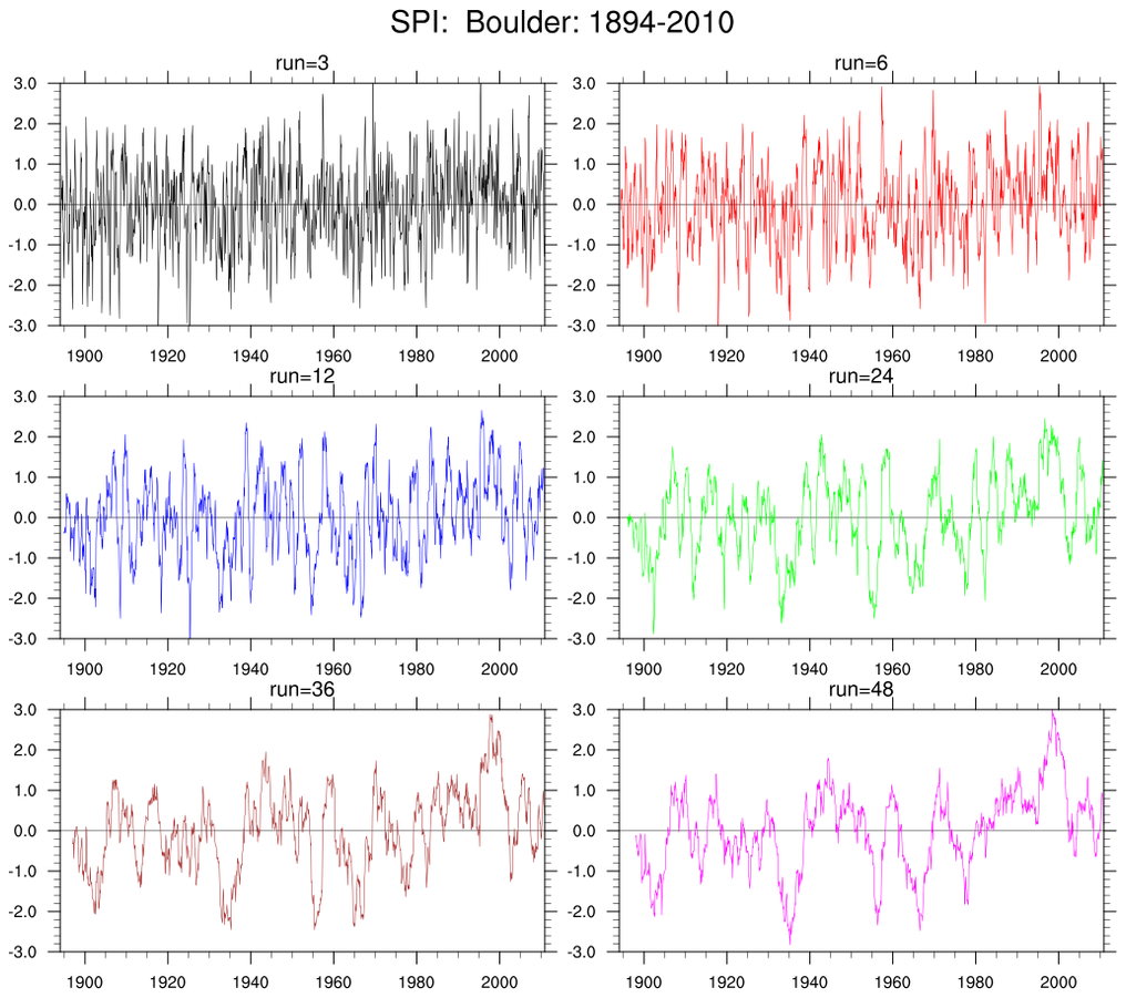
- It can be created for differing periods of 1-to-36 months.
A shortcoming of the SPI, as noted by Trenbert et al (2014):
- "the SPI are based on precipitation alone and provide a measure only for water supply. They are very useful as a measure of precipitation deficits or meteorological drought but are limited because they do not deal with the ET [evapotranspiration] side of the issue."
The SPI is obtained by fitting a gamma or a Pearson Type III distribution to monthly precipitation values. The default implementation of dim_spi_n uses a 2-parameter gamma distribution fit (dim_gamfit_n) where the shape and scale parameters are maximum liklihood estimates as described in
        A Note on the Gamma Distribution
        Thom (1958): Monthly Weather Review, pp 117-122.
                     specifically: eqn 22 for gamma; just above eqn 21
However, there is some variation in the methods used to derive the SPI.
Guttman (1998, 1999) recommends that the Pearson III distribution be used.
Generally, this is likely to give essentially equivalent results to the 2-parameter
gamma distribution fit. In some instances, where monthly and seasonal precipitation
of zero is common, slightly better results.
Generally, monthly precipitation is not normally distributed so a transformation is performed such that the derived SPI values follow a normal distribution. The SPI is the number of standard deviations that the observed value would deviate from the long-term mean, for a normally distributed random variable. One interpretation of the resultant values is:
         [+,-]2.00 and above/below: exceptionally [wet,dry]
         [+,-]1.60 to 1.99: extremely [wet,dry]
         [+,-]1.30 to 1.59: severely [wet,dry]
         [+,-]0.80 to 1.29: moderately [wet,dry]
         [+,-]0.51 to 0.79: abnormally [wet,dry]
         [+,-]0.50:  near normal
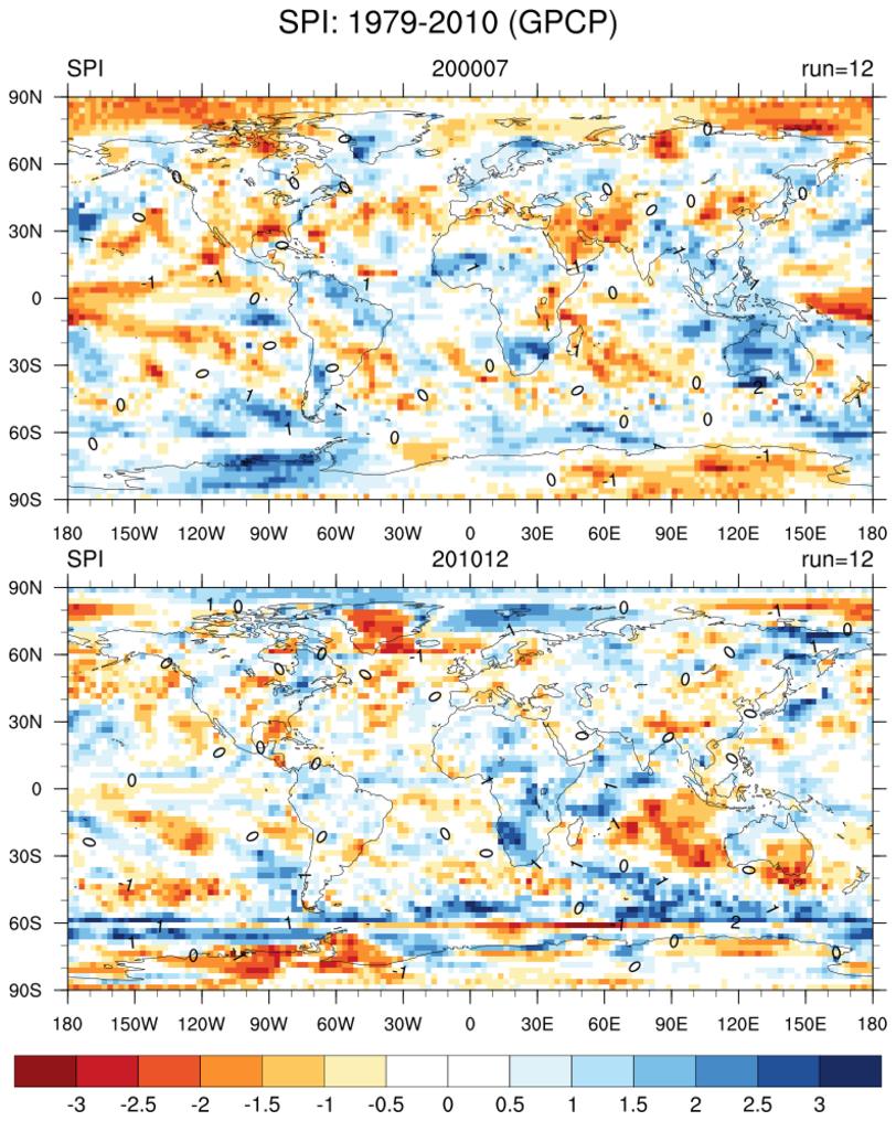
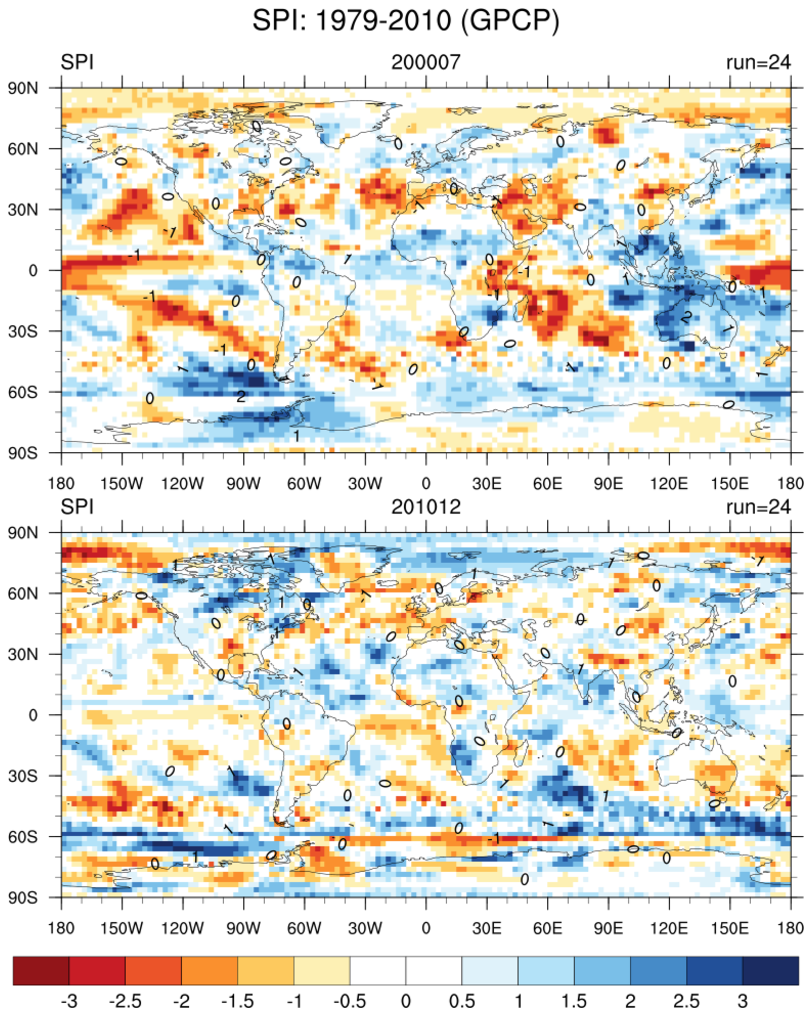
An
explanation of the SPI at different lengths and
sample spatial pattterns
over the USA at different run times are available.
More information can be obtained at the ClimateDataGuide.
References:

      McKee, T.B., N.J. Doesken, and J. Kleist, 1993.
      The relationship of drought frequency and duration ot time scales.
      Eighth Conference on Applied Climatology, American Meteorological Society
      Jan 17-23, 1993, Anaheim CA, pp. 179-186.

      McKee, T.B., N.J. Doesken, and J. Kleist, 1995.
      Drought monitoring with multiple time scales.
      Ninth Conference on Applied Climatology, American Meteorological Society
      Jan 15-20, 1995, Dallas TX, pp. 233-236.

      Guttman, N.B., 1998.
      Comparing the Palmer Drought Index and the Standardized Precipitation Index.
      Journal of the American Water Resources Association, 34(1), 113-121.

      Guttman, N.B., 1999. Accepting the Standardized Precipitation Index: A calculation algorithm.
      Journal of the American Water Resources Association, 35(2), 311-322.

      Trenberth et al (2014)
      Global warming and changes in drought
      Nature Climate Change 4, 17-22;   doi:10.1038/nclimate2067

WMO:
      Handbook of Drought Indicators
      Lincoln Declaration on Drought Indices
      Standardized Precipitation Index User Guide