NCL Graphics: Topographic maps

This page describes various ways to create topographic maps, either by reading them from a binary or NetCDF file, or by importing an existing JPEG image and recreating it.

You can find many free topographic maps (as datasets or images) on the web, including a good site from NOAA:
http://www.ngdc.noaa.gov/mgg/topo/topo.html

There are some high-resolution images available via Nasa's Blue Marble imagery and the 3rd party True Marble:

http://earthobservatory.nasa.gov/Features/BlueMarble/?src=ve
http://www.unearthedoutdoors.net/global_data/true_marble/download

Importing JPEG images

Importing JPEG images into NCL requires converting the JPEG image to a NetCDF file. We use a free tool called "gdal_translate", which is part of the GDAL - Geospatial Data Abstraction software package.

You can download precompiled binaries for Linux and Mac, or you can download the source code and build it yourself.

Building from source requires that you build GDAL with NetCDF support:

./configure --prefix=/path/for/install --with-netcdf=/path/to/netcdf
make all install

/path/for/install and /path/to/netcdf are just placeholders. You need to replace them with the appropriate paths.

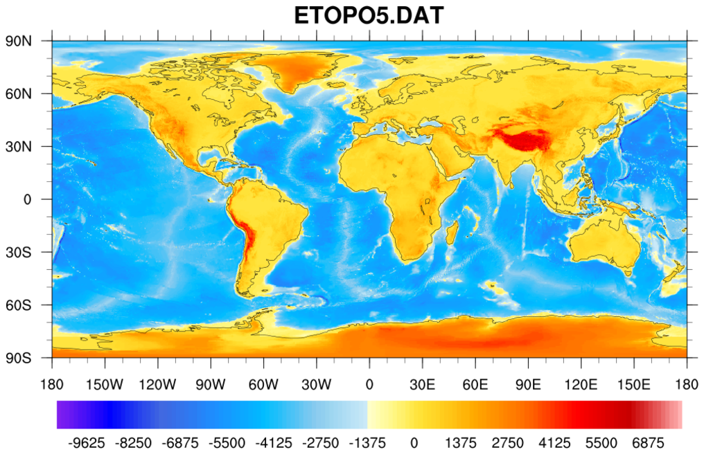
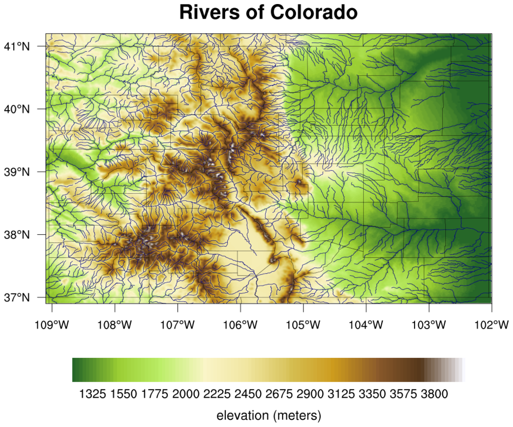
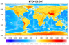topo_1.ncl This script draws a (now deprecated) 5' topographic map using binary data downloaded from http://www.ngdc.noaa.gov/mgg/global/relief/ETOPO5/TOPO/ETOPO5/

This binary file doesn't contain any latitude/longitude values, so these arrays have to be generated in the script. The data comes with a good description of how to read it and create the lat/lon arrays.

The default NCL color map is used just to quickly show what the data looks like.

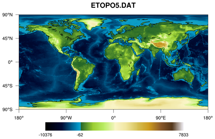
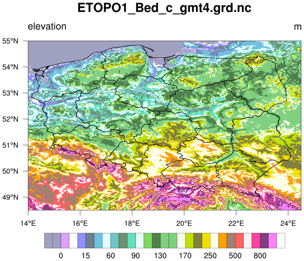
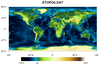topo_2.ncl This script uses the same data as the previous example, except it uses a custom color map. The labelbar is labeled using min/max labels, and a middle level to indicate where the color map was split between ocean and land values.

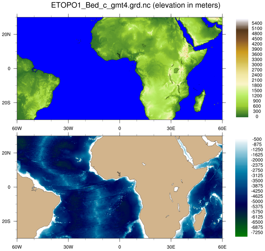
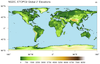topo_3.ncl This script draws a (now deprecated) 2' topographic map using NetCDF data downloaded from http://www.ngdc.noaa.gov/mgg/fliers/01mgg04.html

The cnFillMode resource is set to "MeshFill" for faster plotting. The default "AreaFill" is too slow.

The data are of type "short" with scale_factor and add_offset attributes; the short2flt function is used to unpack the values into a float type.

All elevation values less than -100 are set to missing so there are effectively no contours over the ocean. The ocean is filled in with a light blue.

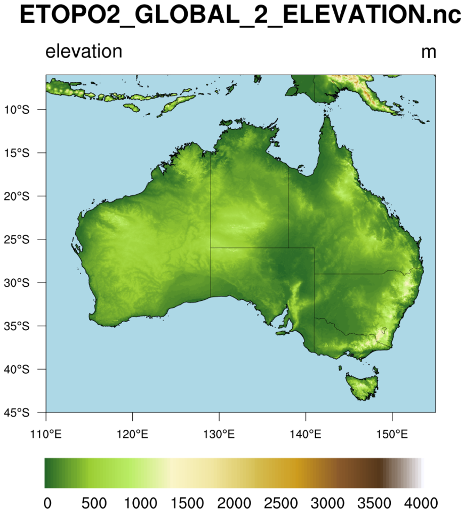
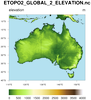topo_4.ncl This script draws a topographic map from the same 2' data as the previous example, except it zooms in on Australia and New Zealand. "RasterFill" is used in place of "MeshFill" for comparison.

topo_5.ncl This script draws a subset of 1' topographic map using NetCDF data downloaded from http://www.ngdc.noaa.gov/mgg/global/relief/ETOPO1/data/bedrock/cell_registered/netcdf/.

Two plots are created in a panel: one showing land elevation values, and one showing ocean elevation values.

topo_6.ncl This script draws a topographic map from the same 1' data as the previous example, except it zooms in on Poland, and uses shapefile data from gadm.org/country to attach the province outlines for Poland.

The color table and levels used were read from a file found at: http://netgis.geo.uw.edu.pl/srtm/wizualizacja.shtml The file can be downloaded here.

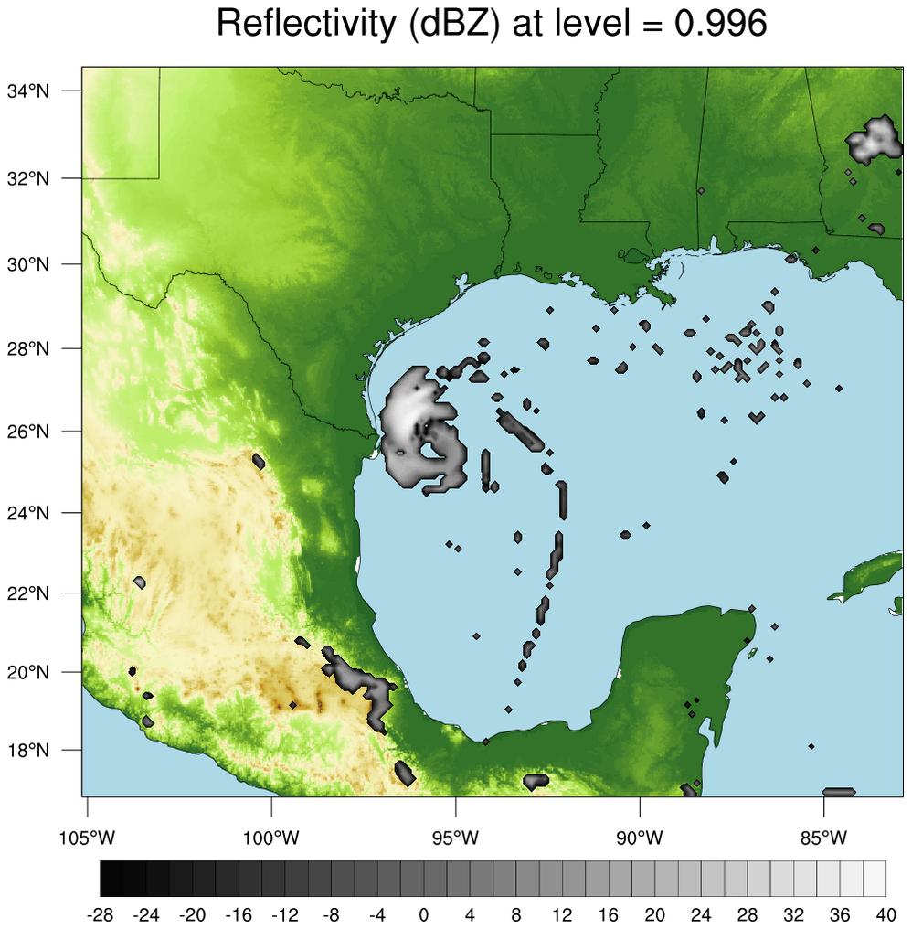
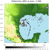topo_7.ncl This example is similar to the WRF "newcolor_10.ncl" example on the new color capabilities page, which shows how to plot "dbz" from a WRF output file on a terrain map. Instead of using the "HGT" variable on the WRF output file to plot terrain, it uses the 2' topo map from examples 3 and 4 above. This gives you a better resolution for terrain, if you need it.

A different colormap is used for dbz, just to show how you can do this. If you set ANIMATE to True, then the script will loop across all levels.

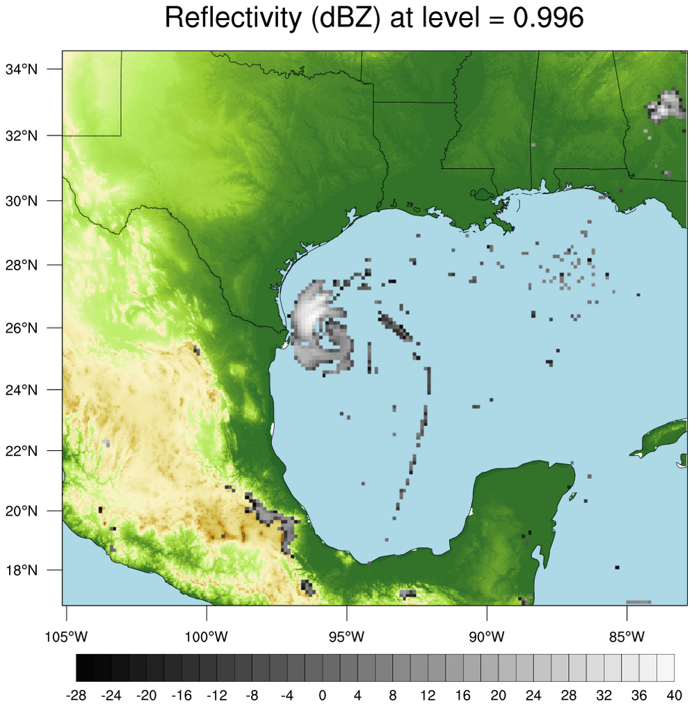
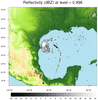topo_raster_7.ncl This example is almost identical to topo_7.ncl above except the reflectivity values are drawn as raster filled contours instead of smooth contours. The point of this example is to illustrate a quirk of using raster fill with transparency. In order to get transparency with raster fill and RGBA values, it's not enough to simply set the alpha value to 0.0. You must also set the color to black as well:

; cmap_r(0,3)  = 0.0             ; This won't work
  cmap_r(0,:)  = 0.0             ; This will work.

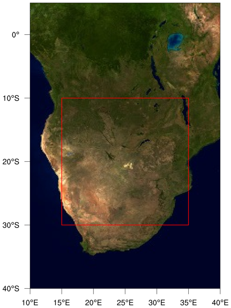
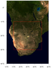topo_8.ncl This script draws a topographic map of Colorado using from 2' data. A shapefile downloaded from http://www.nws.noaa.gov/geodata/catalog/hydro/html/rivers.htm is used to draw the rivers of Colorado.

topo_9.ncl This script is based on the "newcolor_11.ncl" script on the New color capabilities page. It shows how to use NCL to recreate an existing JPEG that contains a topographic map. By doing this, you can then change the map projection, zoom in on it, and/or overlay primitives, as we did here with a red box.

The open source tool gdal_translate was used to convert the jpeg file to a NetCDF file:

  gdal_translate -ot Int16 -of netCDF EarthMap_2500x1250.jpg EarthMap_2500x1250.nc

This example only works for "x11" or "png" output, and not with "ps" and "pdf" output.

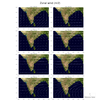
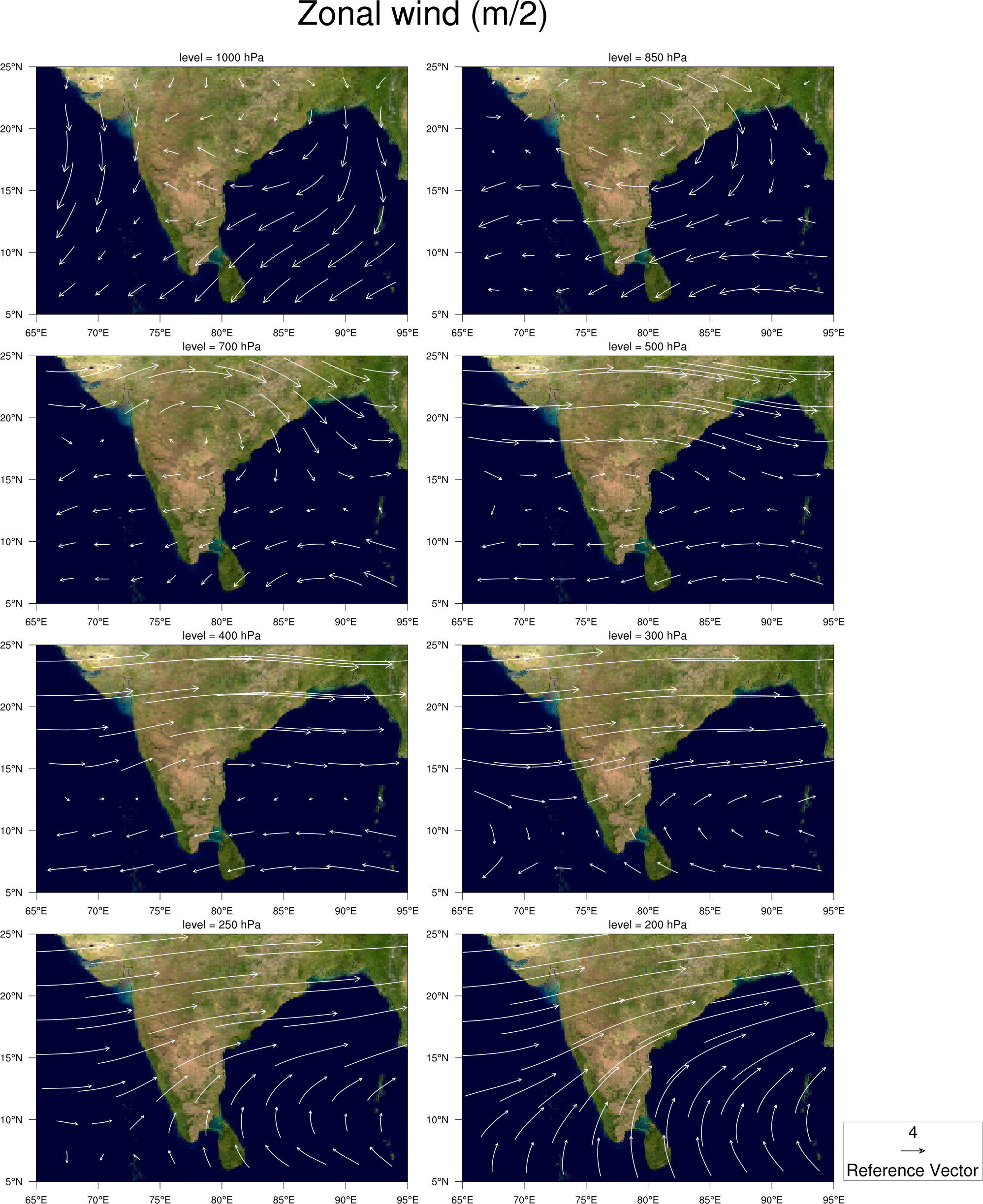
panel_31.ncl: This example shows how to panel vector plots overlaid on topographic maps, and then draw only one vector reference annotation box.

The vector reference annotation box is turned off for all plots except the lower rightmost one, by setting res@vcRefAnnoOn = False for all but that one plot. The box is moved to the outside right of that plot by setting res@vcRefAnnoParallelPosF.

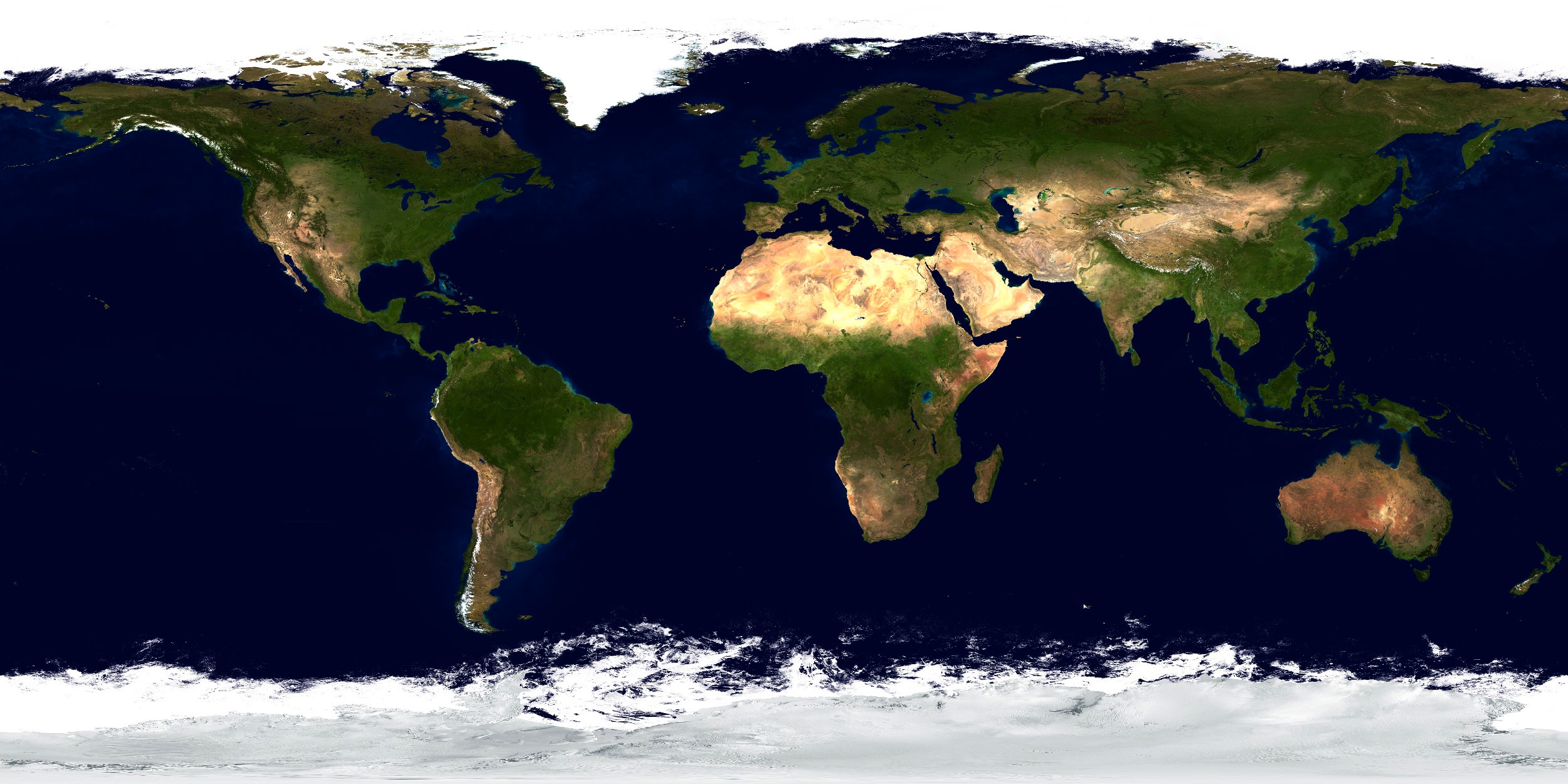
The topographic map is created by reading in a JPEG image. See example newcolor_11.ncl on the RGBA page. This image can be slow to create, so set TOPO_MAP to False in the script if you just want to generate a generic NCL map object (see second thumbnail).