- uv2dvG_Wrap calculates the divergence via spherical harmonics and maintain meta data
- dv2uvg calculates the divergent wind components via spherical harmonics
- uv2vrG_Wrap computes the vorticity via spherical harmonics and maintain meta data
- vr2uvg computes the rotational wind components via spherical harmonics
- uv2dv_cfd computes the divergence via centerd finite differences
- uv2vr_cfd computes the vorticity via centerd finite differences
NCL Home>
Application examples>
Data Analysis ||
Data files for some examples
 wind_1.ncl: First calculates
divergence, then the divergent wind components. Creates a simple
vector plot.
wind_1.ncl: First calculates
divergence, then the divergent wind components. Creates a simple
vector plot.
 wind_2.ncl: First calculates vorticity
and then the rotational wind components. Creates a simple vector plot.
wind_2.ncl: First calculates vorticity
and then the rotational wind components. Creates a simple vector plot.
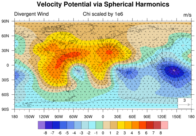
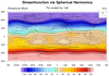 wind_3.ncl: Calculate divergence and vorticity. Then, derive and plot the velocity potential and stream function with
overlays of the divergent and rotational wind components.
wind_3.ncl: Calculate divergence and vorticity. Then, derive and plot the velocity potential and stream function with
overlays of the divergent and rotational wind components.
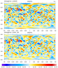 wind_5.ncl:
Example of divergence calculated via spherical harmonics
(uv2dvG) and centered finite differences
uv2dv_cfd. These functions require the grids to be
rectilinear. All spherical harmonic function require global grids.
The centered finite difference function(s) can be used on limited
area grids and allow missing values (_FillValue).
wind_5.ncl:
Example of divergence calculated via spherical harmonics
(uv2dvG) and centered finite differences
uv2dv_cfd. These functions require the grids to be
rectilinear. All spherical harmonic function require global grids.
The centered finite difference function(s) can be used on limited
area grids and allow missing values (_FillValue).

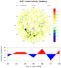
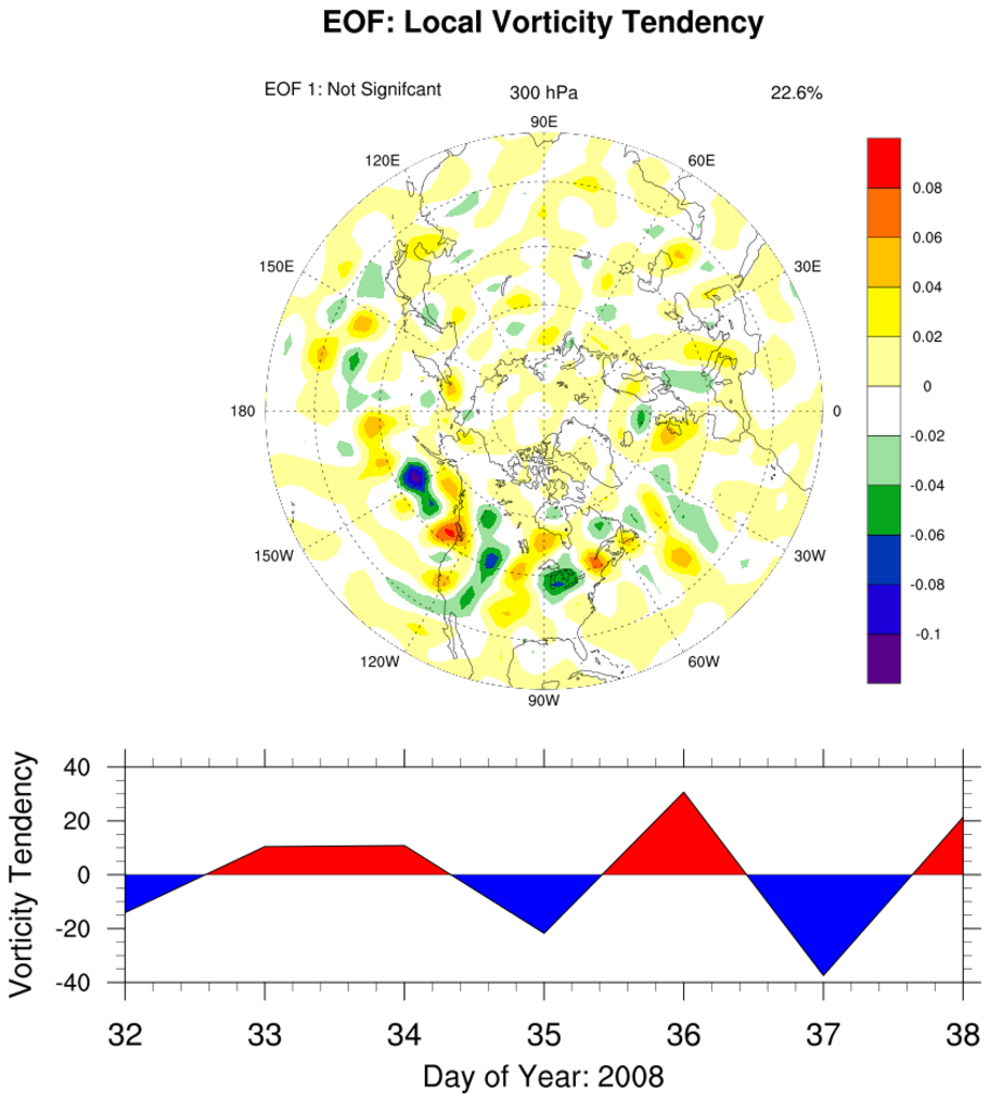
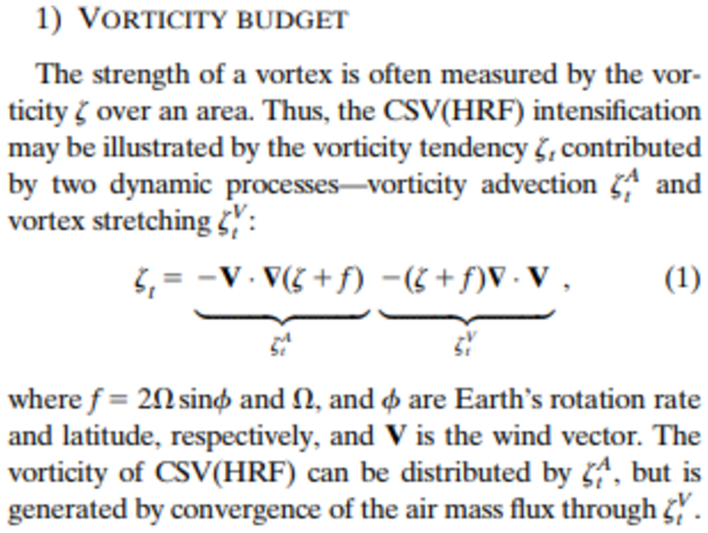
 wind_6.ncl:
Calculate the
local vorticity tendency using spherical harmonics. Spherical harmonics
are used to produce highly accurate gradients. Based upon scale analysis, the
synoptic scale local vorticity tendency can be calculated using the two terms shown
in the rightmost figure. The reference in the wind_6.ncl script provides additional
information. The original code design was to plot an EOF ONLY if it was significant
(see: eofunc_north). However, for this example,
those code lines are commented to illustrate what the EOF plots would look like. Also, only
one EOF plot is presented.
wind_6.ncl:
Calculate the
local vorticity tendency using spherical harmonics. Spherical harmonics
are used to produce highly accurate gradients. Based upon scale analysis, the
synoptic scale local vorticity tendency can be calculated using the two terms shown
in the rightmost figure. The reference in the wind_6.ncl script provides additional
information. The original code design was to plot an EOF ONLY if it was significant
(see: eofunc_north). However, for this example,
those code lines are commented to illustrate what the EOF plots would look like. Also, only
one EOF plot is presented.
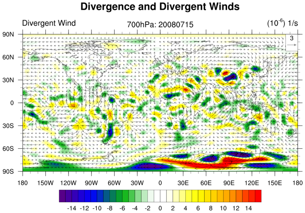
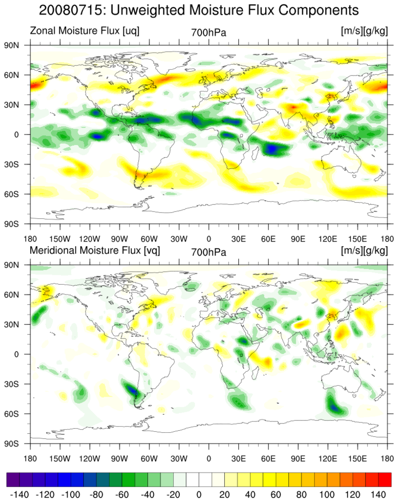
 mfc_div_1.ncl:
Calculate various divergence and moisture quantities including
Vertically Integrated Moisture Flux Convergence (VIMFC).
VIMFC has a high correlation with frontal and convective activity.
Positive values indicate net precipitation.
mfc_div_1.ncl:
Calculate various divergence and moisture quantities including
Vertically Integrated Moisture Flux Convergence (VIMFC).
VIMFC has a high correlation with frontal and convective activity.
Positive values indicate net precipitation.
 mfc_div_2.ncl:
The above MFC equation can be partitioned as follows:
mfc_div_2.ncl:
The above MFC equation can be partitioned as follows:
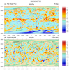
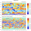
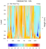
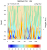 Q1Q2_yanai.ncl:
Using high-frequency [eg: 3/6/12 hourly or daily] data, calculate
apparent-heat-source (Q1) and apparent-moisture-sink (Q2) quantities as described in:
Q1Q2_yanai.ncl:
Using high-frequency [eg: 3/6/12 hourly or daily] data, calculate
apparent-heat-source (Q1) and apparent-moisture-sink (Q2) quantities as described in:
Example pages containing: tips | resources | functions/procedures
NCL: Divergent and Rotational Wind Components
 wind_1.ncl: First calculates
divergence, then the divergent wind components. Creates a simple
vector plot.
wind_1.ncl: First calculates
divergence, then the divergent wind components. Creates a simple
vector plot.
 wind_2.ncl: First calculates vorticity
and then the rotational wind components. Creates a simple vector plot.
wind_2.ncl: First calculates vorticity
and then the rotational wind components. Creates a simple vector plot.

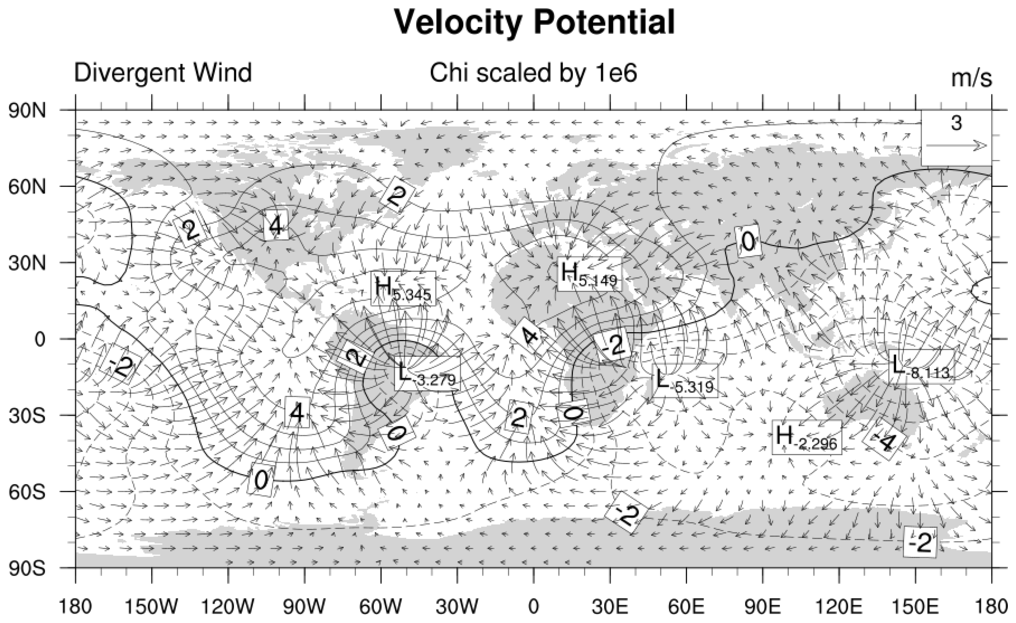
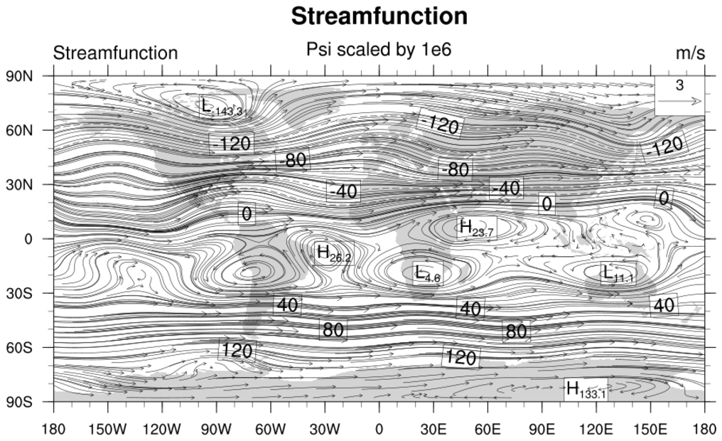
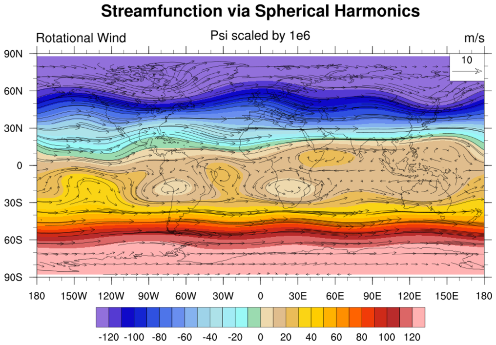 wind_3.ncl: Calculate divergence and vorticity. Then, derive and plot the velocity potential and stream function with
overlays of the divergent and rotational wind components.
wind_3.ncl: Calculate divergence and vorticity. Then, derive and plot the velocity potential and stream function with
overlays of the divergent and rotational wind components.
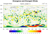
 wind_5.ncl:
Example of divergence calculated via spherical harmonics
(uv2dvG) and centered finite differences
uv2dv_cfd. These functions require the grids to be
rectilinear. All spherical harmonic function require global grids.
The centered finite difference function(s) can be used on limited
area grids and allow missing values (_FillValue).
wind_5.ncl:
Example of divergence calculated via spherical harmonics
(uv2dvG) and centered finite differences
uv2dv_cfd. These functions require the grids to be
rectilinear. All spherical harmonic function require global grids.
The centered finite difference function(s) can be used on limited
area grids and allow missing values (_FillValue).

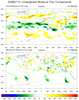
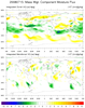
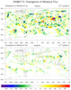
 wind_6.ncl:
Calculate the
local vorticity tendency using spherical harmonics. Spherical harmonics
are used to produce highly accurate gradients. Based upon scale analysis, the
synoptic scale local vorticity tendency can be calculated using the two terms shown
in the rightmost figure. The reference in the wind_6.ncl script provides additional
information. The original code design was to plot an EOF ONLY if it was significant
(see: eofunc_north). However, for this example,
those code lines are commented to illustrate what the EOF plots would look like. Also, only
one EOF plot is presented.
wind_6.ncl:
Calculate the
local vorticity tendency using spherical harmonics. Spherical harmonics
are used to produce highly accurate gradients. Based upon scale analysis, the
synoptic scale local vorticity tendency can be calculated using the two terms shown
in the rightmost figure. The reference in the wind_6.ncl script provides additional
information. The original code design was to plot an EOF ONLY if it was significant
(see: eofunc_north). However, for this example,
those code lines are commented to illustrate what the EOF plots would look like. Also, only
one EOF plot is presented.
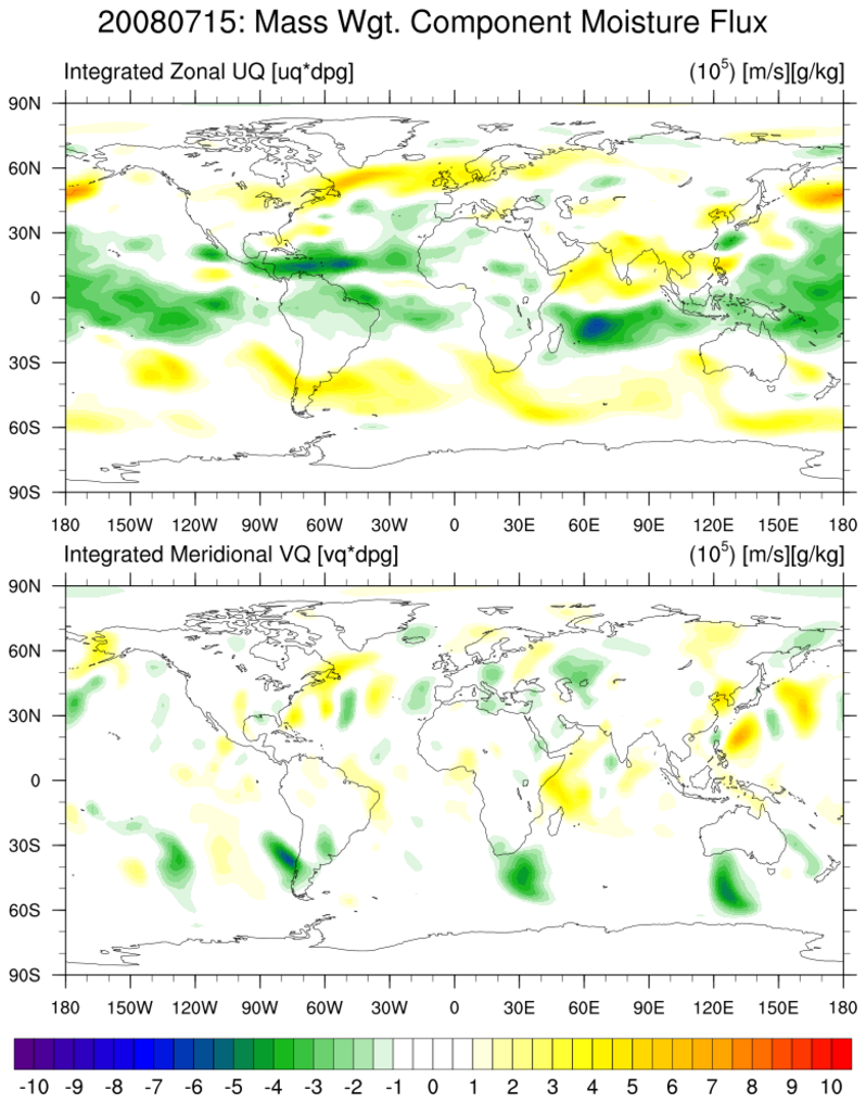
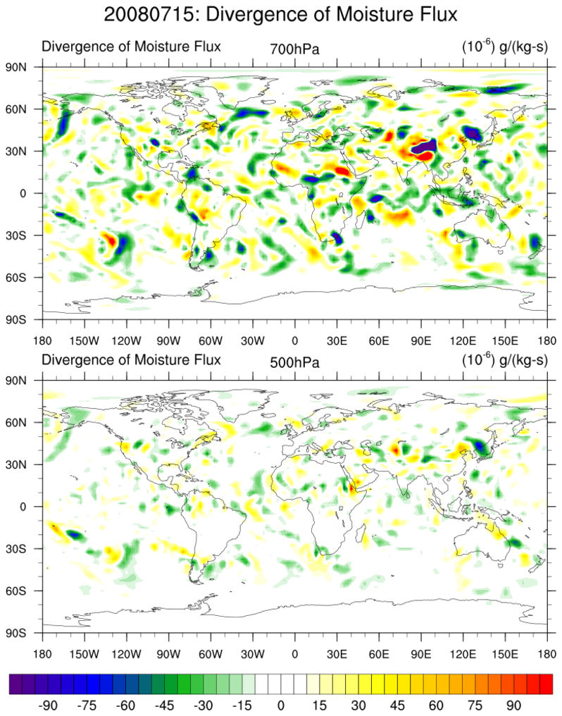
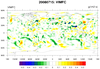
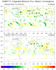
 mfc_div_1.ncl:
Calculate various divergence and moisture quantities including
Vertically Integrated Moisture Flux Convergence (VIMFC).
VIMFC has a high correlation with frontal and convective activity.
Positive values indicate net precipitation.
mfc_div_1.ncl:
Calculate various divergence and moisture quantities including
Vertically Integrated Moisture Flux Convergence (VIMFC).
VIMFC has a high correlation with frontal and convective activity.
Positive values indicate net precipitation.
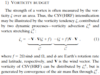
The following equation is implemented within
mfc_div_1.ncl
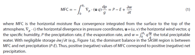
This example uses uv2dvF_Wrap [uv2dvF] because the grid is a global fixed grid. For global gaussian, uv2dvG_Wrap [uv2dvG] should be used. For a regional grid uv2dv_cfd should be used.
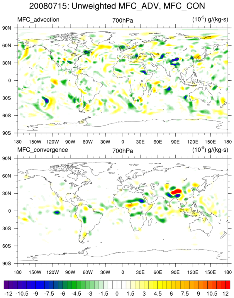
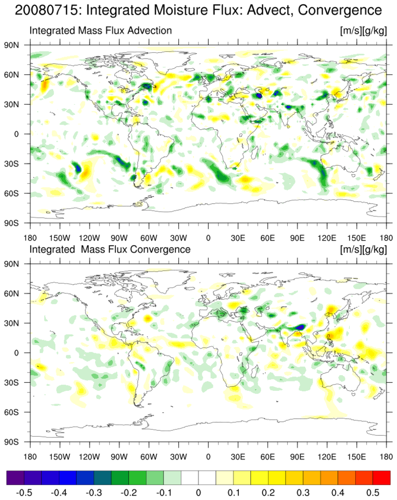
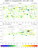
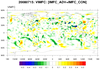
 mfc_div_2.ncl:
The above MFC equation can be partitioned as follows:
mfc_div_2.ncl:
The above MFC equation can be partitioned as follows:
    MFC => Moisture Flux Convergence

    MFC_advect = -(u*(dq/dx)+v*(dq/dy))   ; advect moisture term
    MFC_conv   =  -q*((du/dx)+(dv/dy) )   ; [con/div]ergence term
    MFC        = MFC_advect + MFC_conv
The MFC_advect can be derived using advect_variable
for global rectilinear grids or advect_variable_cfd
for regional rectilinear grids
The MFC_conv can be derived using: uv2dvF_Wrap or uv2dvG_Wrap for global rectilinear grids or uv2dv_cfd for regional rectilinear grids. Then, multiply the derived quantity by specific humidity [q].
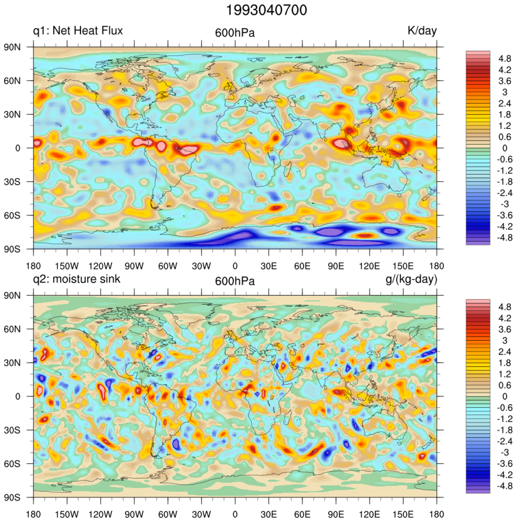
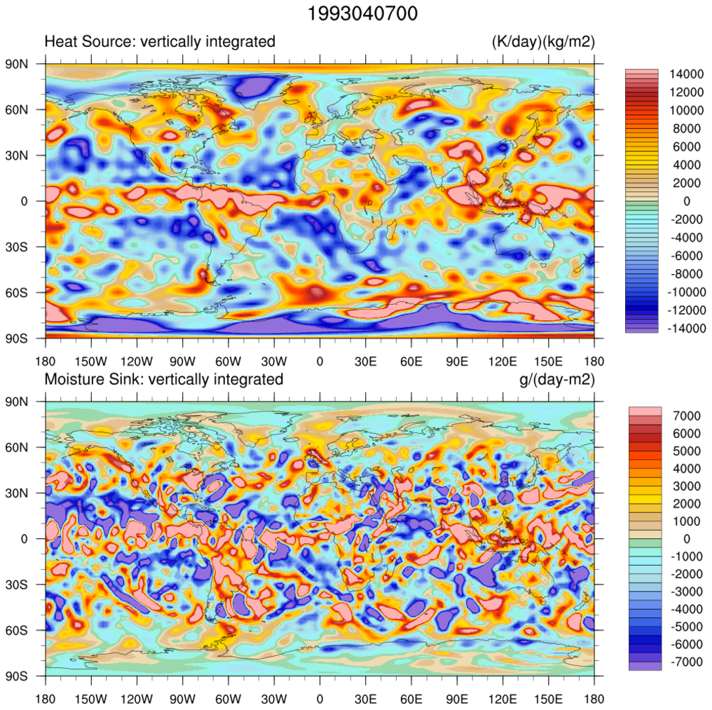

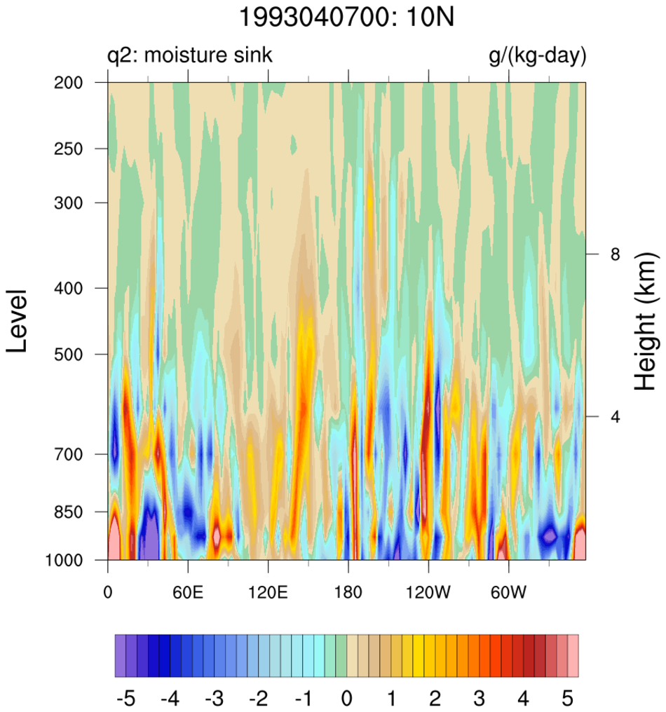 Q1Q2_yanai.ncl:
Using high-frequency [eg: 3/6/12 hourly or daily] data, calculate
apparent-heat-source (Q1) and apparent-moisture-sink (Q2) quantities as described in:
Q1Q2_yanai.ncl:
Using high-frequency [eg: 3/6/12 hourly or daily] data, calculate
apparent-heat-source (Q1) and apparent-moisture-sink (Q2) quantities as described in:
This example uses daily mean data from NOAA/OAR/ESRL PSD, Boulder, Colorado, USA. Specifically, NCEP_Reanalysis 2 daily mean data spanning 3-9 April 1993.
This is a test script. It is not fully tested. The returned quantities are:
         q1 =   (dT/dt) - [omega*static_stability - V.grad(T)]  ; K/day
         q2 = -[(dH/dt) +  V.grad(H) +omega*(dH/dp)]            ; g/(kg-Pa)
    and
         Q1 = Cp*q1     ; apparent Heat Source
         Q2 = Lc*q2     ; apparent Moisture Sink