Non-uniform grids that NCL can contour
This document describes most of the various grids that can now be contoured by NCL. Many of these grids can only be contoured with version 4.2.0.a032 or later. (Go to the download section to get the latest version.)In recent years, many new non-uniform grids have become popular and these are being processed by new algorithms to reduce them to triangle meshes and to contour directly on these triangles, rather than interpolating to a uniform grid and contouring. Contouring and triangulation algorithms have been developed locally by Dave Kennison. Dave Brown of SCD has also developed algorithms based on work of Kennison and work of Jonathan Richard Shewchuk who is in the Computer Science Division at the University of California at Berkeley.
The new triangular mesh functionality gives us access to a huge customer base previously unsupported by NCL. Two important examples include finite element grids which are used by NOAA and other agencies in coastal and tidal hindcast and forecast modeling. It also includes geodesic grids which Dave Randall and colleagues at CSU, in conjunction with the Naval Postgraduate School, are investigating as possible replacements to the current grids used in the CESM.
Here is a list of the grids which are described in detail in subsequent pages. Some of these grids have an NCL example included.
- Lat/Lon
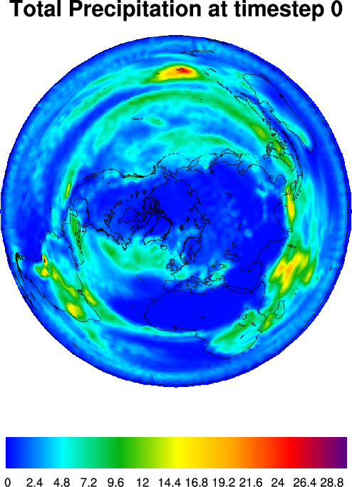
- Geodesic (NCL example)
- Gaussian
- Icosahedral
- ISCCP
- ORCA
- POP
- SEAM (NCL example)
- Triangular mesh (NCL examples)
- Tripole
- Adaptive (NCL example)
- Arpege
This document is primarily a reformatting of a document produced by Dave Kennison.
Lat/lon grids
These are the old traditional rectangular grids, with longitude varying with one of the two dimensions and latitude varying with the other. It is easy to turn such a grid into a triangular mesh by simply splitting each rectangular grid element in half.
Geodesic grids (see also "Icosahedral grids", below)
Most geodesic grids appear to be formed by elaborating an icosahedron; each of the 20 faces of the icosahedron is subdivided into smaller triangles in a more or less obvious way.
Some users think of the geodesic grid as a triangular mesh and others think of it as a bunch of polygonal patches (mostly hexagonal, a few pentagonal), each of which has a vertex of the triangular mesh at its center (i. e., the Voronoi cells).
Randall, Heikes, and Ringler found a way to slightly deform the geodesic grid so as to make all of its triangles have more nearly the same size - the specific techniques have not been detailed.
It is possible to form geodesic grids starting from other regular solids (an octohedron, for example). These are not as common, but here are some sites of interest.
An interesting site containing a bibliography of papers about global grids, compiled for the "International Conference on Discrete Global Grids" by Denis White, at the University of Oregon:
http://www.ncgia.ucsb.edu/globalgrids/bib.html
Another article by White (co-authored with one Kevin Sahr, at Southern Oregon University):
http://bufo.geo.orst.edu/tc/firma/gg/pubs/gdggs98.pdf
It discusses "Discrete Global Grid Systems" based on the various Platonic solids.
A page maintained by Kevin Sahr, with lots of info about DGG's:
http://www.sou.edu/cs/sahr/dgg/
NCL example
| script: geodesic.ncl | ||
|---|---|---|
| 
| 
|
| frame 1 | frame 2 | frame 3 |
Gaussian grids
Paul Swarztrauber is working with these grids. Much like a simple lat/lon grid, but with lines spaced irregularly in latitude.Icosahedral grids (see also "Geodesic grids", above)
These are special cases of geodesic grids.References to "twisted icosahedral grids," are in the literature, but we have not encountered such to date.
There are also references to "stretched icosahedral grids". Examples are at:
http://www.mco.ne.jp/~okirodo/pdf/2608Tomita.pdf
They start with a geodesic grid and then deform it by pulling it towards some point of interest on the globe, so that, near that point, you get more triangles, and, away from that point, you get fewer.
Some names and organizations associated with these grids come from an "International Workshop on the Next-Generation Climate Model":
Detlev Majewski, Deutscher Wetterdienst
Hirofumi Tomita, Frontier Research System
Motohiko Tsugawa, Frontier Research System
Koji Goto, Frontier Research System
John McGregor, CSIRO, Australia
Masaki Satoh, Saitama Institute of Technology
Richard Peltier, University of Toronto, Canada
The Japanese seem to be heavily into these grids.
The site:
http://www.cacr.caltech.edu/Publications/newsletters/update/update1/sect_d.html
contains a paper titled "Argonne Scientists Develop Parallel Method for Simulating Atmospheric Circulation", which makes the point that using an icosahedral grid lends itself to the use of massively parallel computer architectures.
ISCCP grids
"ISCCP" stands for "International Satellite Cloud Climatology Project." The format seems to be an international standard for exchanging global data.
Dennis Shea gave us an example of this grid. It is generated on a cylindrical equidistant projection of the globe. First, horizontal lines are drawn, dividing the projection into 72 strips, each of which is 2.5 degrees of latitude in width. Then, each strip is divided, using vertical lines, into N pieces of equal size, where N is chosen so as to make each piece of the strip have an actual area, on the globe, as close as possible to the area of a 2.5-by-2.5-degree square on the equator. (The strips nearest the equator are divided into 144 pieces, while the strips nearest the poles are divided into only 3 pieces.) Each element of this grid is therefore the little patch on the globe defined by two lines of constant latitude and two lines of constant longitude.
ORCA grids
Christophe Cassou from the Centre National de la Recherche Scientifique (CNRS/CERFACS) in Toulouse uses this grid.The ORCA example we have came from Cristophe Cassou. This grid is common in Europe (particularly in France). The IPSL (Institut Pierre-Simon Laplace) model uses it.
This grid could be described as a tripole grid (see below) that is further modified by the arbitrary displacement of some portions of the grid to achieve finer resolution over areas of interest (typically, ocean areas).
POP grids
These grids may be thought of as rectangular arrays wrapped around the globe in the usual way, with one subscript, call it I, associated with longitude and the other subscript, call it J, associated with latitude, and then deformed in such a way as to move the top edge of the array to a circle centered somewhere other than over the North Pole (typically, over Greenland or Canada) and the bottom edge of the array to a circle that is centered on the South Pole, but lies entirely within Antarctica. The lines defined by the rows and columns of the rectangular arrays are locally orthogonal to each other.
The site "http://www.cgd.ucar.edu/csm/models/ocn-pop/grids.shtml" is of interest. "POP" stands for "Parallel Ocean Program" and it was developed at Los Alamos.
POP grids are used extensively locally in oceanographic and ice models.
Here is a site with a lot of useful information, both historical and descriptive:
http://climate.lanl.gov/Models/POP/
Technically, the POP grids are called "displaced-pole" grids, as opposed to "tripole" grids.
SEAM (Spectral Element Atmospheric Model) grids
Used heavily in the HOMME (High-order Multiscale Modeling Environment).
Some names:
Steve Thomas, NCAR
Jim Edwards, IBM & NCAR
Rich Loft, NCAR
Bill Spotz, NCAR
Joseph J. Tribbia, NCAR
Aimee Fournier, NCAR & University of Maryland
Mark Taylor, Los Alamos National Laboratory
Houjun Wang, NCAR & University of Maryland
Ferdinand Baer, University of Maryland
Some Web sites:
http://www.cgd.ucar.edu/gds/wanghj/taylor/doe/seam.html
http://www.nersc.gov/news/annual_reports/annrep99/25sh_baer.html
http://www.osti.gov/scidac/updates2004/ber_9.html
http://www.seam.com/p_visiseam.htm
http://www.cs.sandia.gov/capabilities/ClimateSimulation/MPSAtmosphereModel.html
Houjun Wang gave us two different examples, both of which are developed from a cube embedded inside the globe. The examples shown on the first Web site above show various techniques for constructing the initial set of quadrilaterals and for subdividing some of the quadrilaterals into smaller quadrilaterals in regions where higher resolution is desired.
What characterizes a SEAM grid, though, is the way in which the set of quadrilaterals representing the globe (or some portion thereof), are subdivided into "spectral elements" that are used in implementing the model you're writing. I ran into a paper describing the use of spectral element methods on the triangles of a geodesic grid.
NCL example
| script: seam.ncl | |||||
|---|---|---|---|---|---|
| 
| 
| 
| 
| 
|
| frame 1 | frame 2 | frame 3 | frame 4 | frame 5 | frame 6 |
Triangular meshes:
Simona Bordoni, Department of Atmospheric Sciences, UCLA - satellite "swaths". These are actually defined by rectangular arrays of latitudes and longitudes from which some points (generally speaking, those over land) are missing; these are much easier to handle as triangular meshes, so that the missing portions of the mesh can simply be omitted.
Tom Gross, NOAA/NOS/CSDL/MMAP, also program manager for the Chesapeake Community Model, Chesapeake Research Consortium (tom.gross@noaa.gov) - Chesapeake Bay example.
Brett Estrade, Naval Research Laboratory, Stennis Space Center, Mississippi (estrade@nrlssc.navy.mil) - North Carolina coastline.
Daniel Sheltraw, University of New Mexico (sheltraw@unm.edu) - arbitrary object in 3-space. His particular application involved drawing contours on an isosurface of a magnetic field.
NCL examples
| script: ctnccl.ncl | script: chspkbay.ncl | ||
|---|---|---|---|
| 
| 
| 
|
| frame 1 | frame 2 | frame 1 | frame 2 |
Tripole grids
These grids are somewhat like the POP grids, but the top row of the rectangular array, instead of mapping to a circle on the globe, maps to a degenerate circle forming a line passing through the North Pole. The end points of this line are two of the three "poles" of the grid, the other one being at the South Pole. Tripole grids seem to be used by the same people who use POP grids and they are the starting point for the ORCA grids.
Adaptive grids
We have worked with an adaptive grid that comes from Christiane Jablonowski with ECMWF. (cjablono@ucar.edu). Christiane's grid is constructed using boundary lines which are all either horizontal or vertical on a cylindrical equidistant projection of the globe. First, the rectangular area covered by the projection is divided into smaller rectangles, all of which are the same size. Some (but not all) of these rectangles are subdivided into four smaller rectangles of equal size, and some (but, again, not all) of those are subdivided into even smaller rectangles of equal size.NCL example
| script: adaptive.ncl
data file: fvgcm_amr.delp.000240.000.nc | |||
|---|---|---|---|
| 
| 
| 
|
| frame 1 | frame 2 | frame 3 | frame 4 |
ARPEGE grids:
We have plotted such a grid that came from from Christophe Cassou. An organization that seems to use these is "Meteo-France".This grid is similar to the ISCCP grid, but with somewhat finer resolution. Also, the grid is rotated with respect to the globe so as to put its poles somewhere other than at the North and South Pole.
This grid is being handled using Dave Brown's adaptation of a code called "Triangle," written by Jonathan Richard Shewchuk.
NCL example
| script: arpege.ncl | |
|---|---|

| 
|
| frame 1 | frame 2 |