NCL Home>
Application examples>
Data sets ||
Data files for some examples
Example pages containing:
tips |
resources |
functions/procedures
NCL: High Resolution Precipitation:
CMORPH, PERSIANN, TRMM,
GPM, GPCP, CPC_Famine, ST4
NCL Comments
Generally, the examples below process only one file.
To process multiple files would require only minor additions
to the sample codes.
        dir  = "./"               ; input directory
        fili = systemfunc("cd "+dir+" ; ls root*") ; 'root' is unique
        nfil = dimsizes(fili)

        do nf=0,nfil-1
            :
            ; change all fili to fili(nf)
            :
        end do
------------------------------------------------------------------------
Reading "big endian" and "little endian" binary file types
is readily accomplished via
        setfileoption("bin","ReadByteOrder","BigEndian")
    or
        setfileoption("bin","ReadByteOrder","LittleEndian")
------------------------------------------------------------------------
Interpolating high spatial/temporal resolution precipitation fields,
is best accomplished via area_conserve_remap or the
ESMF software.
Note: The area_hi2lores has been deprecated as of NCL Version 5.2.0.
However, it is used here for backward compatibility.
All of the basic interpolation functions have "_Wrap" versions which
preserve and create appropriate meta data:
area_conserve_remap_Wrap,
linint2_Wrap,
area_hi2lores_Wrap (deprecated).
If netCDF creation is desired and file space is a concern,
it may be best to "pack" the precipitation values.
Using pack_values
will create a file half the size of those created
using float values. Some precision is lost but is not important here.
------------------------------------------------------------------------
Often, precipitation variables contain N-hourly accumulated
totals, where N=1 or 3 or 6 or 12. A common question:
Given hourly precipitation (eg, 0Z, 1Z, 2Z, ..., 23Z, 0Z, ...),
how can (say) 6-hourly (0Z, 6Z, 12Z, 18Z) totals be calculated?
Please see Example 5 of the dim_sum_n function.
The CMORPH examples use the
cnFillPalette resource introduced in NCL 6.1.0 (Oct 28, 2012).
This facilitates associating different color schemes and contour levels.
NOTE: There is one more color than there are contour levels.
  res@cnLevelSelectionMode = "ExplicitLevels"
  res@cnLevels             = (/0.1,1,2.5,5,10,15,20,25,50,75/) ;   ; 10 contour values
  res@cnFillPalette        = (/"Snow","PaleTurquoise","PaleGreen"\ ; 11 contour colors
                              ,"SeaGreen3" ,"Yellow","Orange"    \
                              ,"HotPink","Orange","HotPink","Red"\
                              ,"Violet", "Purple", "Brown"       /)
Subsequently, if different contour levels and colors are needed, the 'cnLevels' and 'cnFillPalette'
resources would have to be deleted because the array sizes are different.
NCL's
:= syntax, introduced in NCL 6.1.1 (Feb 2013) can be used.
  res@cnLevelSelectionMode = "ExplicitLevels"
  res@cnLevels          := (/5,10,20,30,40,50/)                     ; 6 contour values
  res@cnFillPalette     := (/"Snow","PaleGreen","Yellow" \          ; 7 contour colors
                            ,"Orange","Red","Purple", "Brown"/)
The GPM files are HDF5. These use 'groups' a new data structure for HDF.
 cmorph_1.ncl
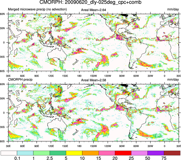
:
Read a big endian binary file containing daily total
precipitation at 0.25 degree resolution. The plot contains
the merged satellite precipitation and the
Climate Prediction Center's morphed estimates. Create netCDF.
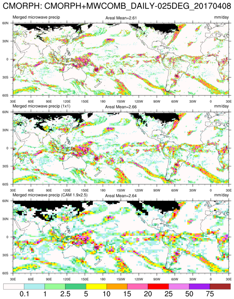
 cmorph_2.ncl
:
Interpolate the 0.25 gridded data to (a) 1x1 degree resolution
and (b) the Community Atmosphere Model (CAM) 1.9x2.5
degree grid. Create netCDF.
 cmorph_trilbar_2.ncl
:
This example is the same as cmorph_2, except that the labelbar ends are triangular. This is accomplished by setting
the resource
lbBoxEndCapStyle to "TriangleBothEnds".
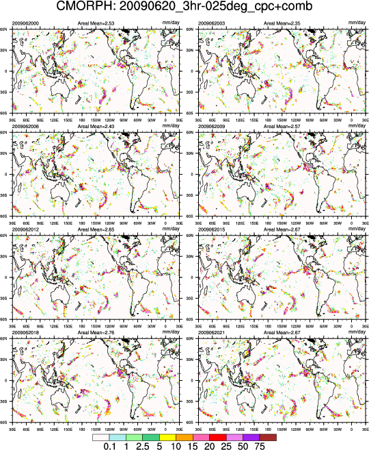
 cmorph_3.ncl
:
Read the 3-hourly CMORPH grids for one day: plot and create netCDF.
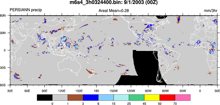
 persiann_1.ncl
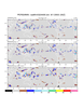
:
Read a big endian binary file containing 3-hourly
precipitation at 0.25 degree resolution. The geographical
extent is 60N to 60S. Create a
packed netCDF
using the
pack_values function.
This creates a file half the size of those created
using float values. Some precision is lost but is not important here.
The plot style here mimics that used at the
PERSIANN WWW site.
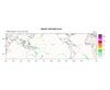
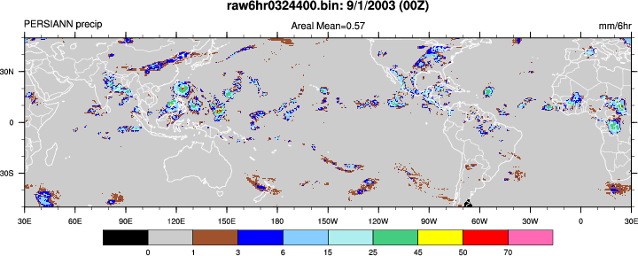
 persiann_2.ncl
:
Analogous to the previous example but it uses
a big endian binary file containing 6-hourly
precipitation at 0.25 degree resolution. The geographical
extent is 50N to 50S. Create packed netCDF.
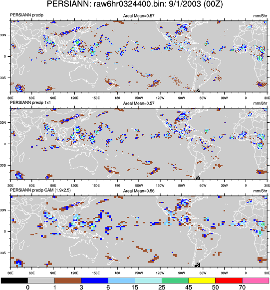
 persiann_3.ncl
:
Interpolate the 6-hourly 0.25 gridded data to (a) 1x1 degree resolution
and (b) the Community Atmosphere Model (CAM) 1.9x2.5
degree grid. Create packed netCDF.
 persiann_4.ncl
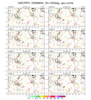
:
(a) Read one or more binary file(s) [3000x9000]; (b) Explore data; (c) Increase workstation workspace; (d) Plot ; (e) Create netCDF-4."
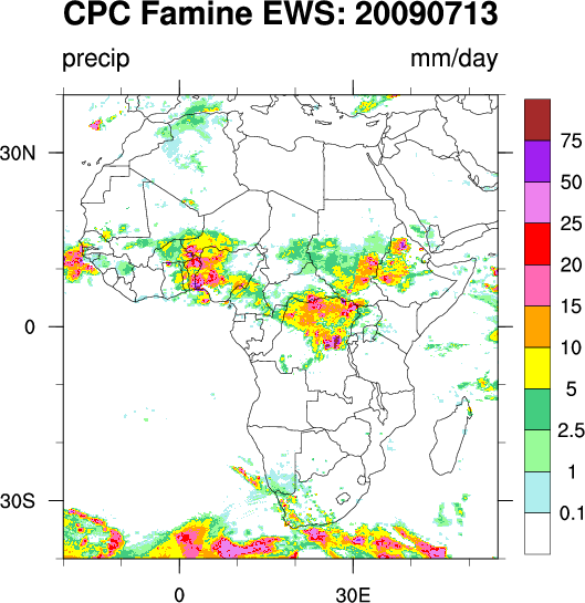
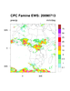 cpcFamine_1.ncl
:
Read a big endian binary file containing daily total
precipitation at 0.1 degree resolution. The
daily precipitation estimates are obtained by merging
GTS gauge observations and 3 kinds of satellite estimates:
GPI,SSM/I and AMSU. Create netCDF.
For this file, the areal average is 1.3 mm/day.
The maximum value is 265.4 mm/day.
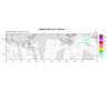
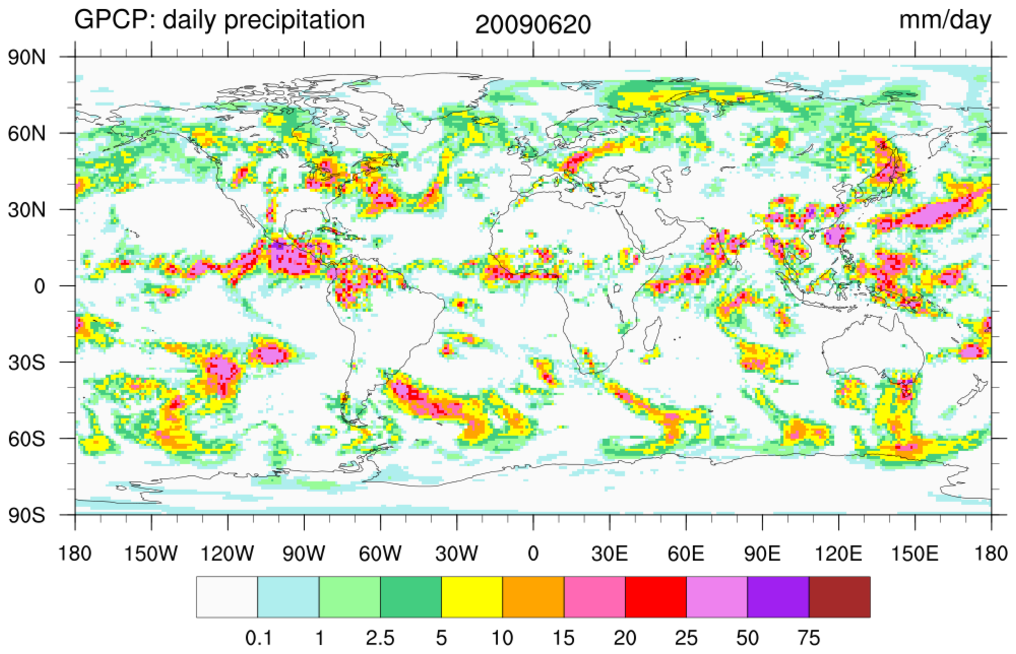
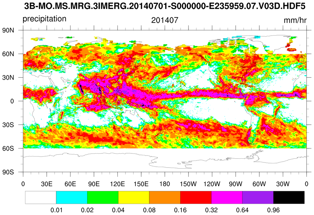
 gpcp_4.ncl
:
Plot GPCP-1DD for a user specified date.
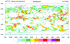
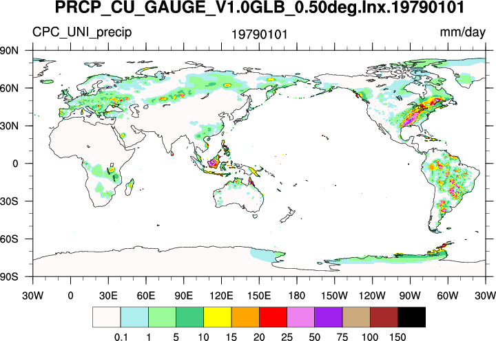
 cpcuni_1.ncl
:
Read one or more CPC_Unified binary files. Optionally: (a) Create netCDF and/or (b) plot the data.
If multiple files are being read and corresponding netCDF files are created, there is an
option to concatenate (combine) all the netCDF into one file use the netCDF Operator (NCO)
ncrcat. This is invoked
by creating a string containing the desired command and, then,
executing the command via the
system procedure.
The plots have a contour max of 150 mm/day. However, many files contain values much greater
than this: 250, 300, etc. The script prints the min and max values for each file.
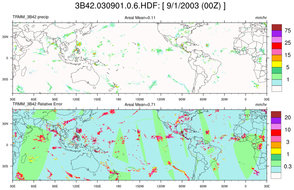
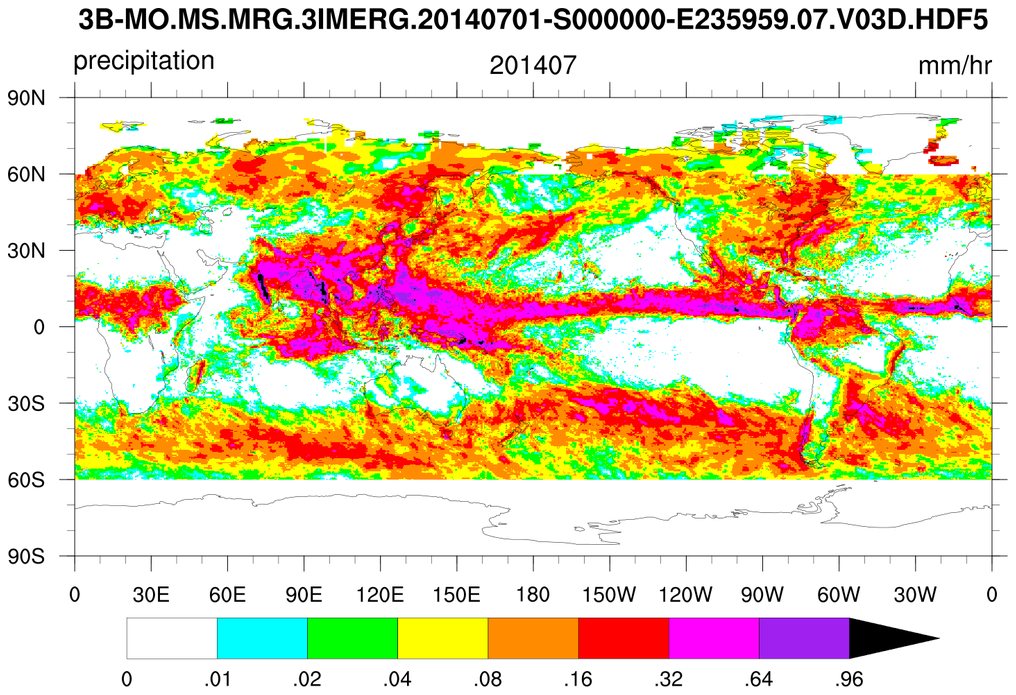
 trmm_1.ncl
:
Read a HDF file containing 3-hourly
precipitation at 0.25 degree resolution. The geographical
extent is 40S to 40N. Create a
packed netCDF
using the
pack_values function.
This creates a file half the size of those created
using float values. Some precision is lost but is not important here.
The HDF file is classifed as a "Scientific Data Set" [HDF-SDS].
Unfortunately, it does not contain the geographical coordinates
or temporal information. The former must be obtained via
a web site while the time is in the file name.
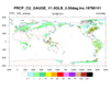
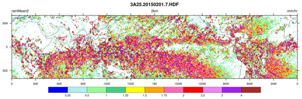
 trmm_3A25_1.ncl
:
Read a HDF-SDS file containing monthly precipitation rates derived
from the 3A25 precipitation algorithm. The 'rainMean2'
variable is at 0.25 degree resolution.
The HDF file is classifed as a "Scientific Data Set" [HDF-SDS].
Unfortunately, it does not contain the geographical coordinates
or temporal information. The former must be obtained via
a web site while the time is in the file name.
Climate and Forecast meta data is manually added.
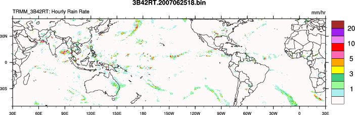
 trmm_3B42RT_1.ncl
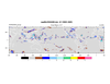
:
The 3B42
RT (
Real
Time) product is a big-endian binary file containing
variables of mixed types: type character, type short and type byte.
NCL can be used to read the data but it is a bit cumbersome because
NCL's binary read functions only read one variable type. They lack the
necessay 'granularity' to partition the different variable
types. The approach is to read the
entire file as a single type
and extract the appropriate information.
The same record must be read for
each type specification.
Hence, the user must keep track of the byte counts.
The trmm_3B42RT_1.ncl script reads one or more 3B42RT
binary files. It unpacks the data (see description in the script) and
creates a netCDF file for each input binary file containing the unpacked values.
It also plots a simple image. Note: for this plot, all negative precipitation
values were set to _FillValue.
trmm_3B42RT_2.ncl:
Read one or more 3B42
RT binary files and create a CF-1.0
convention conforming netCDF file with the original numeric types
(short and byte). The character record is included as global
attributes. In addition, a reference is added. A
sample
ncl_filedump
(same as
ncdump -h)
is
here. It
is
slightly larger than the original binary file because it
contains additional information (time/date, lat/lon, reference).
 trmm_3B40RT_1.ncl
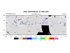
:
The 3B40
RT (
Real
Time) product is a big-endian binary file containing
variables of mixed types: type character, type short and type byte.
NCL can be used to read the data but it is a bit cumbersome because
NCL's binary read functions only read one variable type. They lack the
necessay 'granularity' to partition the different variable
types. The approach is to read the
entire file as a single type
and extract the appropriate information.
The same record must be read for
each type specification.
Hence, the user must keep track of the byte counts.
The trmm_3B40RT_1.ncl script reads one or more 3B40RT
binary files. It unpacks the data (see description in the script) and
creates a netCDF file for each input binary file containing the unpacked values.
It also plots a simple image. Note: for this plot, all negative precipitation
values were set to _FillValue.
trmm_3B40RT_2.ncl:
Read one or more 3B40
RT binary files and create a CF-1.0
convention conforming netCDF file with the original numeric types
(short and byte). The character record is included as global
attributes. In addition, a reference is added. A
sample
ncl_filedump
(same as
ncdump -h)
is
here. It
is
slightly larger than the original binary file because it
contains additional information (time/date, lat/lon, reference).
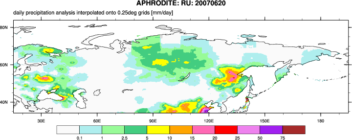
 aphro_1.ncl
:
Read an APHRODITE netCDF file containing daily mean rain rates and create simple regional plot.
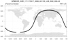
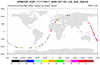
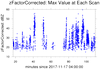
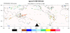
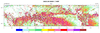
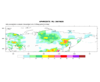
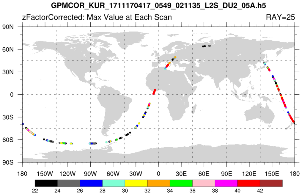
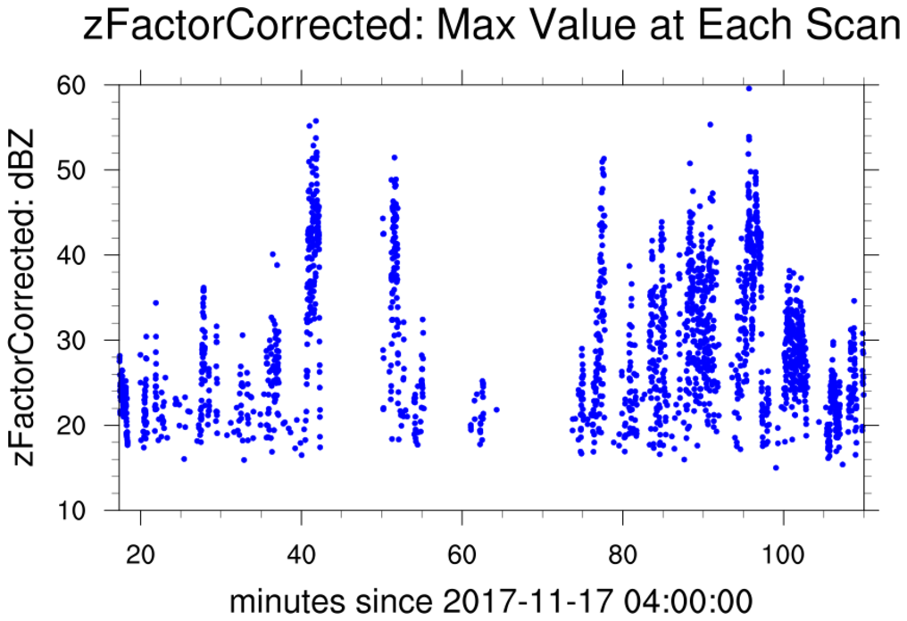
 gpm_2.ncl
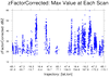
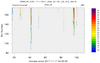
:
Read a GPM HDF5 file containing swath data from the COR satellite.
Read the 'zFactorCorrected' radar values with dimensionality:
[nscan | 7935] x [nray | 49] x [nbin | 176]
Each 'nscan' corresponds to a unique time.
The nray represent 49 samples perpendicular to the trajectory.
The nbin represent 176 vertical' samples at each scan and ray..
There are
many missing values.
Plot the trajectory data in different ways: (a) trajectory only;
(b) polymarkers colored by the maximum value at each scan (time);
(c) time series using polymarkers for maximum values at each time (scan);
(d) same as (c) but plotting latitude and longitude as the abscissa; and,
(e) plotting a contour cross-section.
Create a CF-conforming time variable using
cd_inv_calendar.
Use
nice_mnmxintvl and
stat_dispersion
to explore the data and set plot resources.
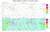
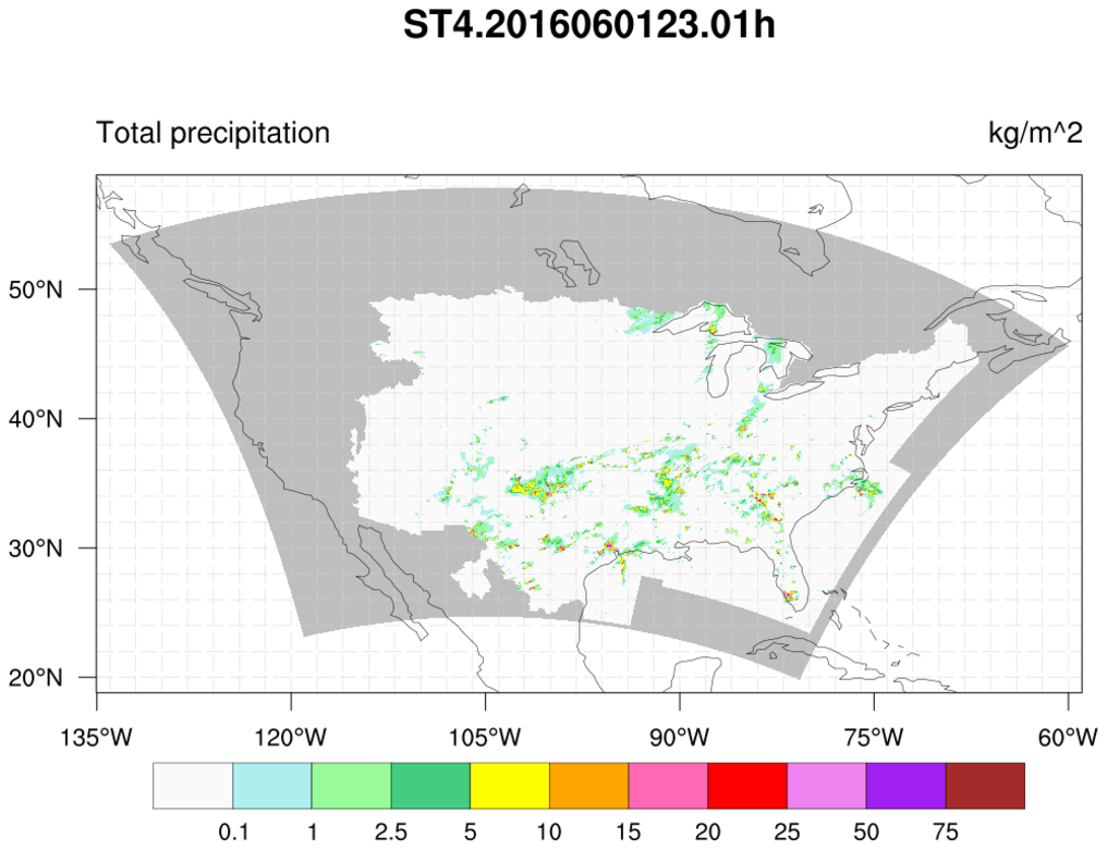
 ST4_1.ncl
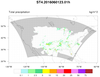
:
Read an
NCEP Stage IV
regional hourly/6-hourly multi-sensor (radar+gauges) precipitation analyses on a 4km grid.
Plot and explicitly show grid locations with missing values (light gray).
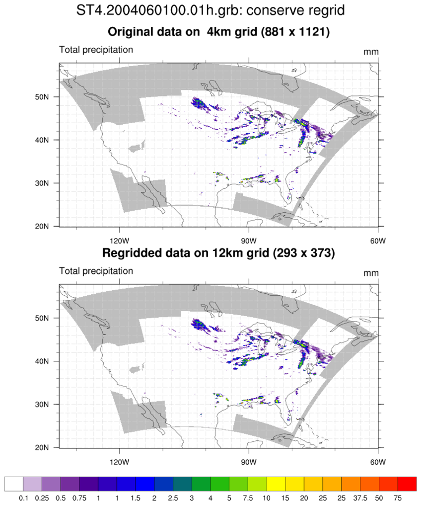
 ST4_2.ncl
:
Read an
NCEP Stage IV
regional hourly/6-hourly multi-sensor (radar+gauges) precipitation analyses.
Use
ESMF conservative interpolation to regrid from 4km resolution to 12km resolution.
Plot and explicitly show grid locations with missing values (light gray).


