NCL Graphics: Contour Raster Mode

Raster contours (cnFillMode = "RasterFill") are created by individually assigning colors to the elements of a 2D array of rectangular cells. With raster contours, only solid fill is possible and therefore resources related to pattern fill have no effect.

Raster fill can be much faster than the default "area fill". If the raster contours look too "blocky", you can try setting cnRasterSmoothingOn = True.

Prior to version 6.2.0, the raster fill mode did not support transparency. For that reason, areas outside the grid or with missing values were filled in the background color (usually white). Now these areas are set by default to the Transparent color index just as they are using the other fill modes. This allows for more flexibility in overlaying a raster fill plot over other plot objects such as a background map. It is easy enough to obtain the look generated by previous versions of NCL if you set the resource cnMissingValFillColor to "white".

If raster and area contours are not generating what you want, you can try "cell fill": cnFillMode = "CellFill". Cell-filled contours are created by drawing filled polygons whose edges are defined by the borders between adjacent grid cells.

For examples of cell fill, see the 2D vertical coordinates or ORCA pages.

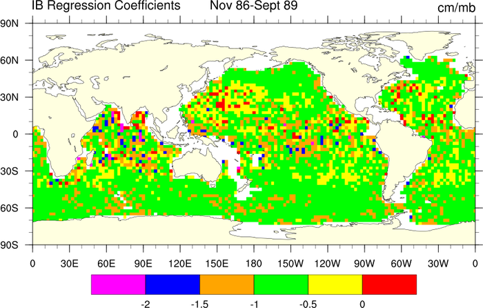
raster_1.ncl: A typical raster plot.

cnFillMode = "RasterFill" turns on raster fill mode. When this is on, it is better to turn off the contour lines by setting cnLinesOn = False.

To fill the continents with color and an outline,
cnLineDrawOrder = "Predraw", cnFillDrawOrder = "Predraw", cnFillOn = True, are set. Without these, only the continental outlines are drawn.

mpLandFillColor = "LightYellow", chooses which color out of the colormap to draw the continents. The default is light grey.

cnFillOn = True, also turns on the label bar. If cnFillMode = "RasterFill", alone is selected, then you will get color with no label bar.

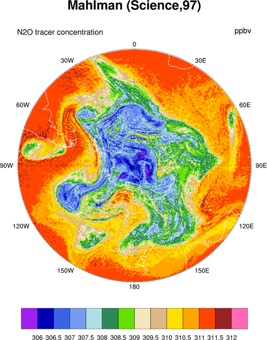
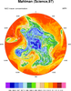raster_2.ncl: A reproduction of a figure published in a 1997 Science article. This plot does not have the "boxy" appearance of a raster plot because the grid cell size is very small.

mpGeophysicalLineColor = "white", changes the continental outline color to white.

gsnPolar = "SH", selects the southern hemisphere for a polar plot.

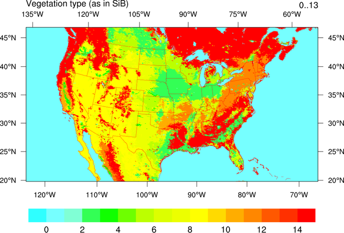
raster_3.ncl: This vegetation raster plot is generated using 2-dimensional latitude and longitude coordinate values. These values are attached as attributes to the data (veg@lat2d and veg@lon2d), since traditional coordinate array syntax can't be used (these have to be 1-dimensional).

The gsnRightStringOrthogonalPosF and gsnLeftStringOrthogonalPosF resources are used to move the two subtitles up from the plot.

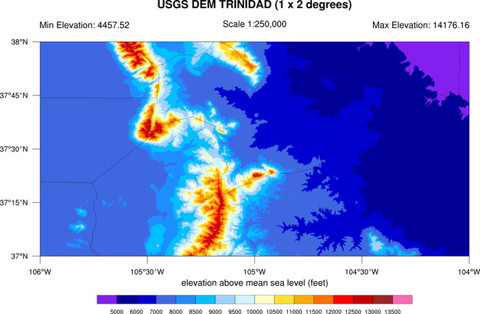
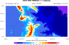raster_4.ncl: This script shows how to create a topographic map using a raster contour graphic colored by elevation.

This example is also available as a Python script using PyNGL to generate the graphics and PyNIO to read the data from a netCDF file. See the PyNGL gallery for a pointer to the script.

This example was written by Mark Stevens of NCAR.

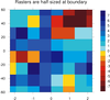
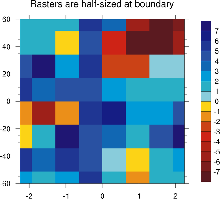
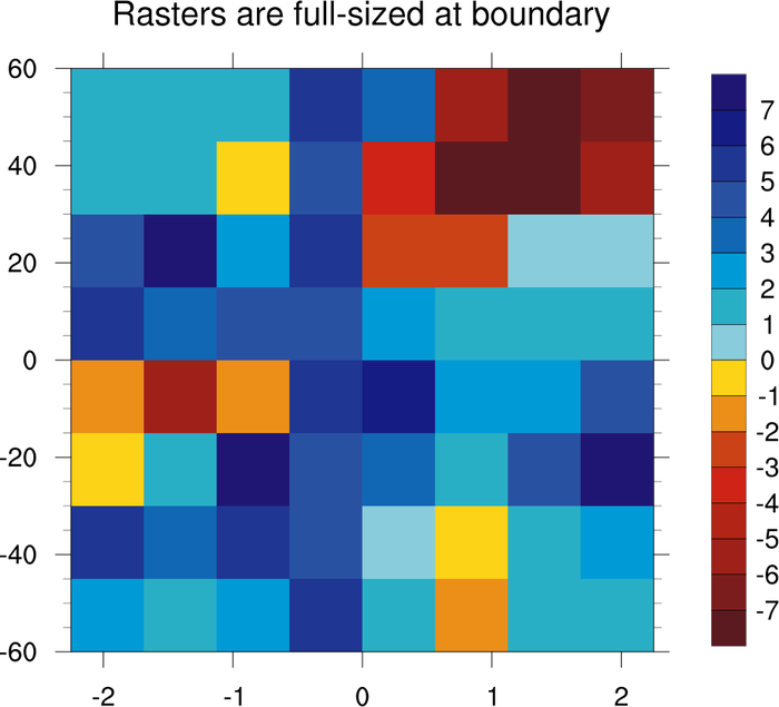
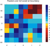raster_5.ncl: This script shows how to force full-sized raster cells at the X and Y axis boundaries. You need to have coordinate arrays that are one element longer than the dimensions of your data. This forces the data values to represent the center of a grid, rather than the corners of a grid.

For example, if your array is dimensioned 8 x 8, then your coordinate arrays must have 9 elements each. To contour this kind of data, you must set the sfXArray and sfYArray resources to these two arrays.

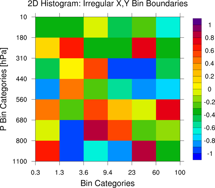
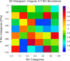raster_6.ncl: This is a slight variation of the previous example. It is a two-dimensional histogram where the X and Y bin boundaries are irregularly spaced.

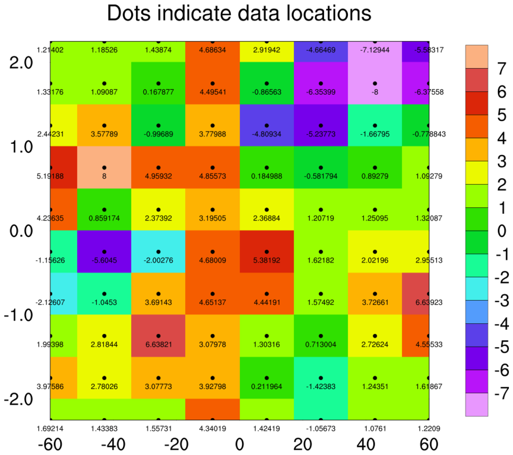
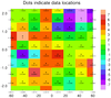raster_7.ncl: This is yet another variation of example 5. This is to illustrate how a raster plot is created. NCL internally contructs a box around each data value, and fills that box in the appropriate color indicated by your contour levels and the color map.