Example pages containing: tips | resources | functions/procedures
NCL Graphics: Slices
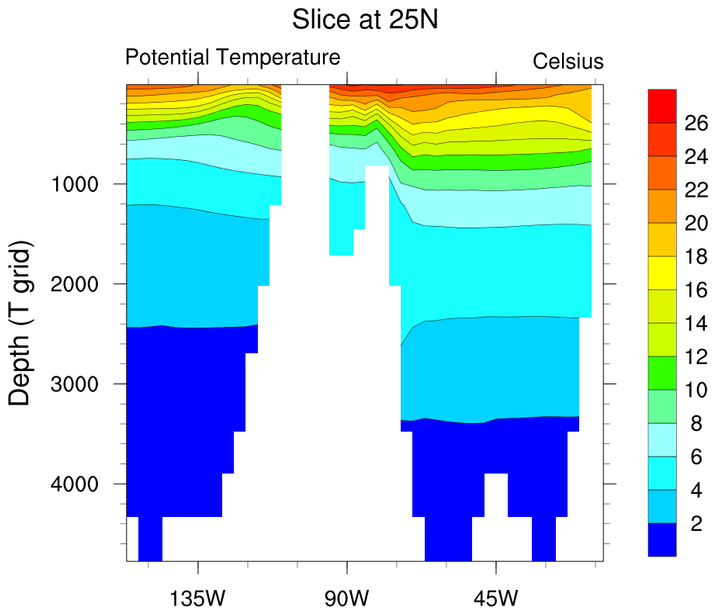 slice_1.ncl: A slice of an ocean
model.
slice_1.ncl: A slice of an ocean
model.
sfXArray= lon_t, and
sfXArray= z_t/100 set the
vectors to be used for the x and y axis respectively.
Most vertical axis are irregular. We can display them as a linear axis by setting gsnYAxisIrregular2Linear = True
Frequently, we will need to reverse the y axis. This is done by setting trYReverse = True
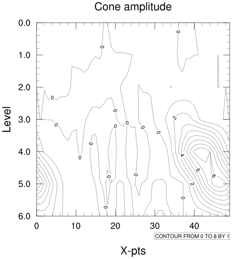 slice_2.ncl: A slice of data that
contains no geophysical coordinates
slice_2.ncl: A slice of data that
contains no geophysical coordinates
Because this data has no lat/lon coordinate arrays, we use gsn_contour which does not look for geophysical coordinates.
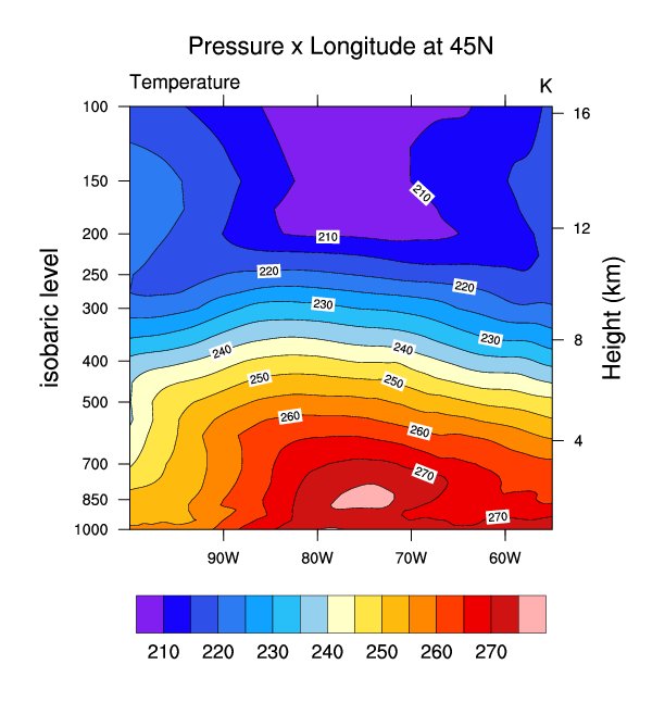
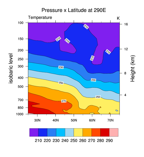
 narr_5.ncl:
This script uses an ESMF generated weight file
(See: ESMF Example 30) to efficiently regrid a
source NARR curvilinear grid to a rectilinear grid. Then three cross sections are plotted:
(a) pressure x longitude; (b) pressure x latitude; and, (c) pressure x user_speciied_set_of_points.
For this example the user specified latitude/longitude locations lie along a great circle path
between two user specified locations (See: gc_latlon). They could be
latitude/longitude locations along a (say) cold front.
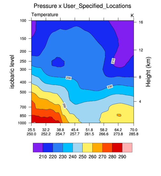
narr_5.ncl:
This script uses an ESMF generated weight file
(See: ESMF Example 30) to efficiently regrid a
source NARR curvilinear grid to a rectilinear grid. Then three cross sections are plotted:
(a) pressure x longitude; (b) pressure x latitude; and, (c) pressure x user_speciied_set_of_points.
For this example the user specified latitude/longitude locations lie along a great circle path
between two user specified locations (See: gc_latlon). They could be
latitude/longitude locations along a (say) cold front.
ESMF Example 30 was run twice: bilinear and conservative interpolation. Bilinear interpolation would generally be appropriate for any reasonably smooth variable. Conservation interpolation would be recommended for interpolating flux quantities and variables that can be fractal (eg precipitation).
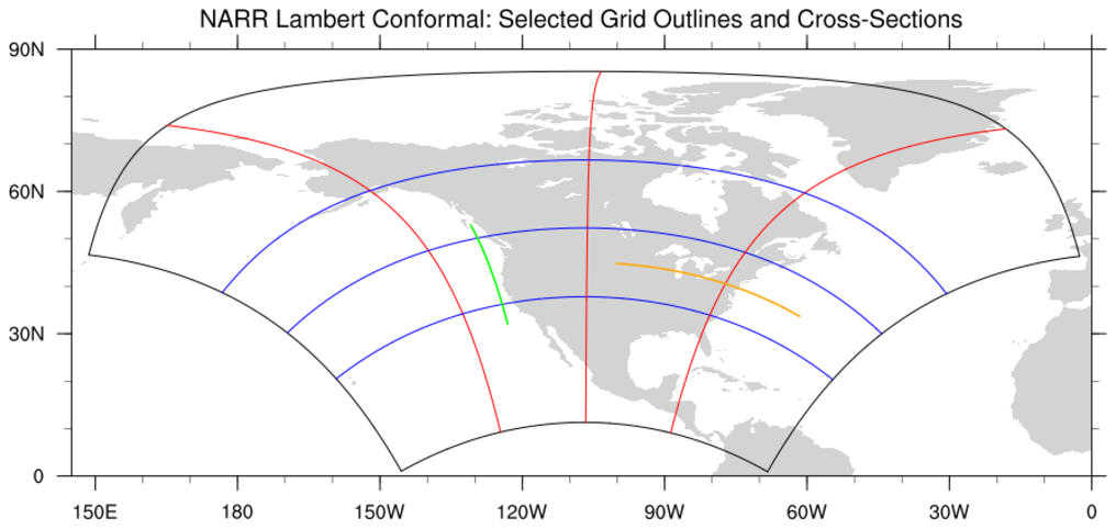
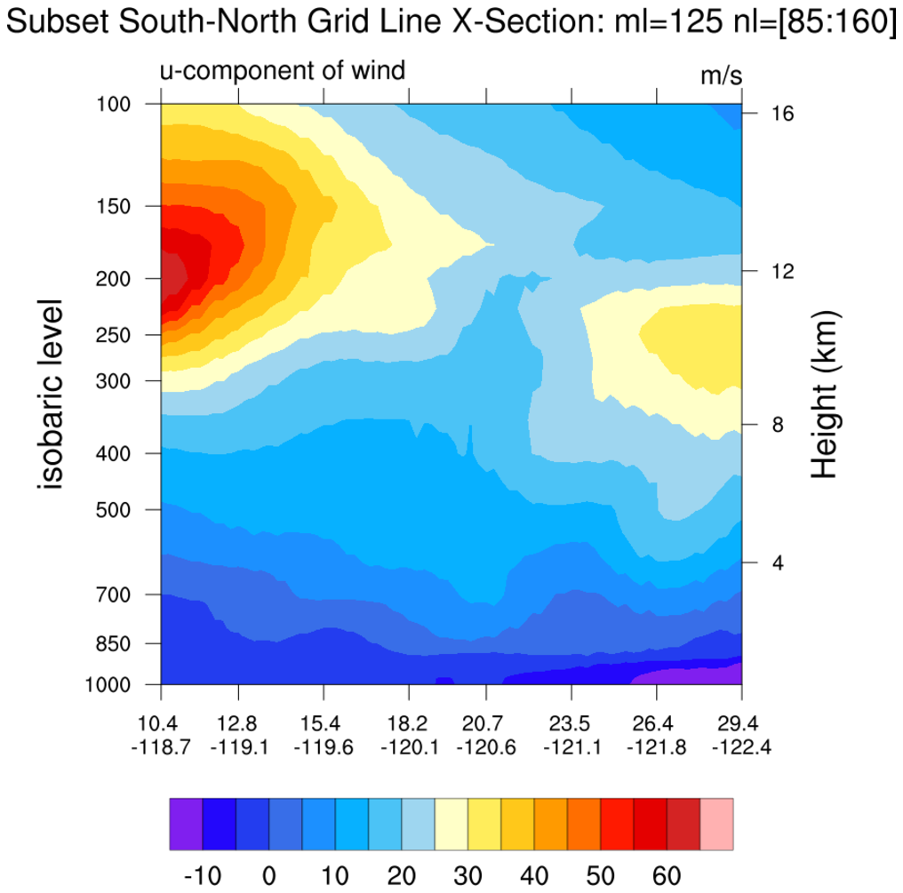
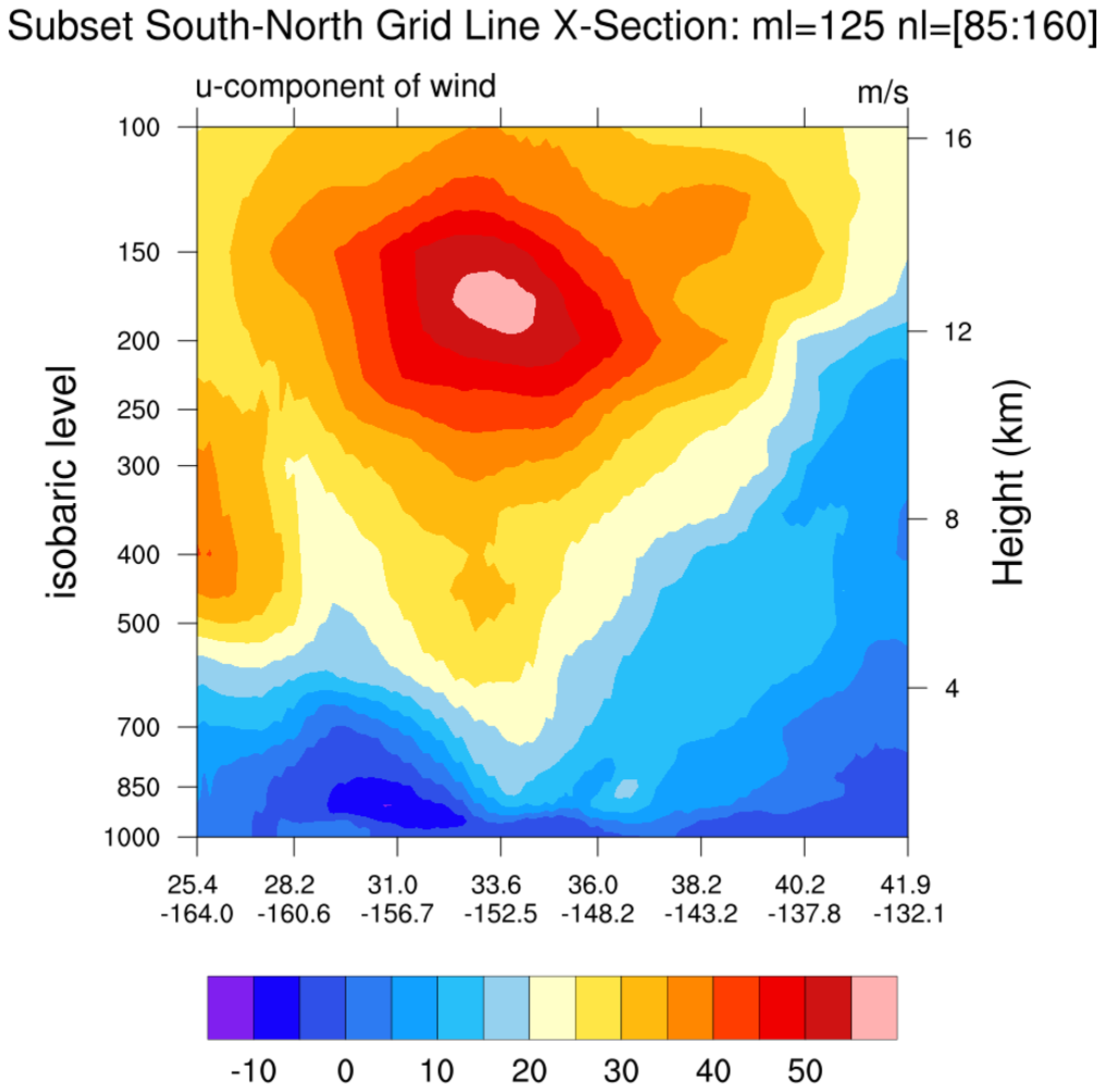 narr_6.ncl:
The NARR grid is curvilinear. This means that the grid point locations require
two-dimensional latitude and longitude arrays. The leftmost figure shows the
north, south, west and east boundaries (black outline);
selected east-west grid lines (blue); selected north-south grid lines (red); and,
user specified subsets of grid lines. Sample 'grid line following' cross sections
are created.
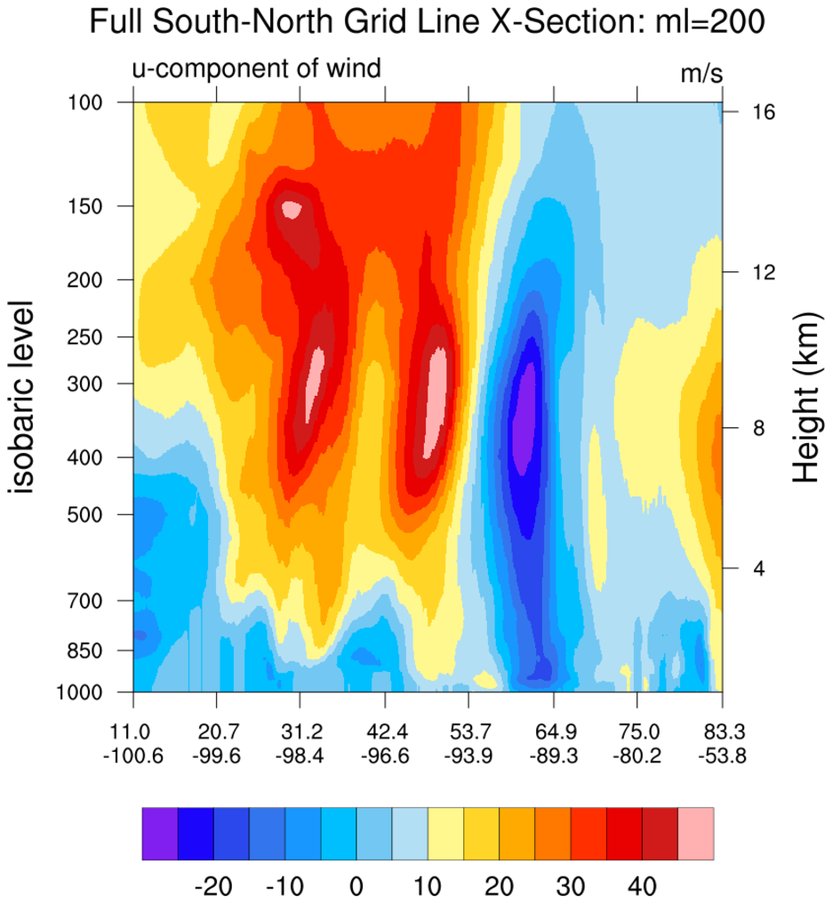
narr_6.ncl:
The NARR grid is curvilinear. This means that the grid point locations require
two-dimensional latitude and longitude arrays. The leftmost figure shows the
north, south, west and east boundaries (black outline);
selected east-west grid lines (blue); selected north-south grid lines (red); and,
user specified subsets of grid lines. Sample 'grid line following' cross sections
are created.