NCL Graphics: TIGGE Project

TIGGE Project

TIGGE, the THORPEX Interactive Grand Global Ensemble, is a key component of THORPEX: a World Weather Research Programme to accelerate the improvements in the accuracy of 1-day to 2 week high-impact weather forecasts for the benefit of humanity. Centralized archives of ensemble model forecast data, from many international centers, will be used to enable extensive data sharing and research.

The following examples show how to plot multiple ensemble members on one plot (a spaghetti plot), how to calculate an ensemble average, and how to calculate a grand ensemble from data on 5 different grids (from 5 different modeling centers).

All TIGGE data files are in GRIB1/GRIB2 format. In the examples below, the file extension ".grib2" is appended to each TIGGE file. NCL recognizes the following case-insensitive extensions for GRIB files: ".grb" , ".grib", ".grb1", ".grib1", ".grb2", "grib2". The actual file need not have the specified GRIB extension. By default, NCL will look for the exact file name as specified in the addfile function. If that file name is not found, NCL will look for the file name without the file extension and treat it as a GRIB file.

Note that users can use ncl_filedump to look at the contents of a GRIB1/GRIB2 file. The output from using ncl_filedump on a ecmf TIGGE file can be found here.

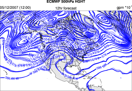
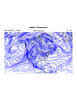
tigge_1.ncl: Demonstrates how to draw a spaghetti plot showing Z500 from the first 10 ECMWF ensemble members for a 12-hr forecast. The key to creating a spaghetti plot is to set gsnDraw and gsnFrame to False, and to use the overlay function to overlay one plot on top of another. After all the plots are overlaid, draw and frame must be called. In this example, a map is created first with titles, and then 10 contour fields (from the first 10 ensemble members) are overlaid on the map.

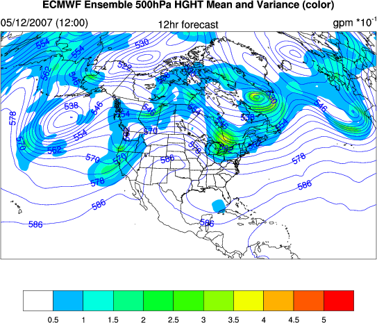
For the second plot, an ensemble average is created by using dim_avg_Wrap to average across the 51 ECMWF ensemble members. The variance (or spread) amongst the individual ensemble members is also calculated by using dim_variance_Wrap. gsn_csm_contour_map_overlay is used to overlay the mean plot over the variance plot.

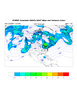
tigge_2.ncl: A spaghetti plot showing the 564dm (@500hPa) contour from all 51 ECMWF ensemble members (blue lines) and the ensemble average of the 51 members (thick red line).

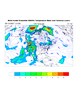
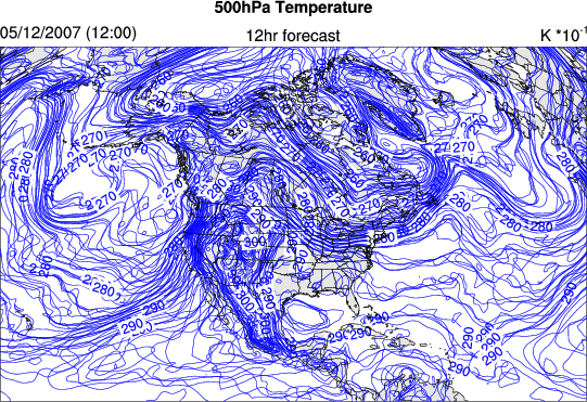
tigge_3.ncl: A spaghetti plot showing the T@500hPa ensemble average from each of the 5 modeling centers participating in the TIGGE project.

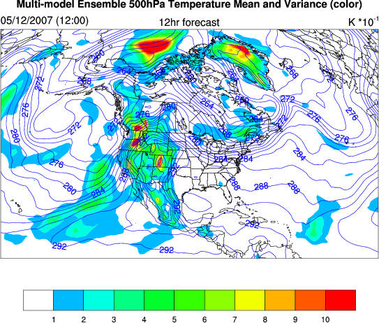
For the second plot, the 5 modeling center ensembles are averaged to form a grand ensemble. The variance (or spread) amongst the five ensemble members is also calculated by using dim_variance_Wrap.

Four of the ensembles (babj, ecmf, egrr, and kwbc) are regridded to the rjtd ensemble resolution for this calculation. (The rjtd ensemble resolution was chosen because it has the lowest resolution.) The function linint2_Wrap was used for the regridding. Note that linint2_Wrap expects the input/output latitude/longitude grids to be monotonically increasing. The input/output latitudes must run from south->north, and the longitudes must run from west->east. The ecmf, babj, kwbc, and rjtd grids had latitudes that ran from north->south, and they were easily flipped by using the syntax "::-1" when the data were being read into NCL.

The grand ensemble formed in this example was calculated by averaging the 5 modeling centers ensemble averages. This method ensures that each modeling center's ensemble receives equal weight in the grand ensemble. Another method used to form a grand ensemble is to average across each individual ensemble member from each of the 5 modeling centers. In this case, that would result in averaging 15 (babj)+ 51 (ecmf)+ 24 (egrr)+ 21 (kwbc)+ 51 (rjtd) = 162 ensemble members. Note that this method results in those models with the largest number of ensemble members (ecmf/rjtd) having more of an effect on the grand ensemble than those models that have fewer ensemble members (babj/egrr/kwbc).

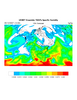
tigge_4.ncl: Shows the UKMET ensemble average 12hr forecast of the specific humidity field at 700hPa using color shading.