NCL Graphics: Subsetting / extracting data based on lat/lon values

latlon_subset_1.ncl: Data on a rectilinear grid is the easiest to subset, as you can use coordinate subscripting to extract the region of interest.

To find out if your data is on a rectilinear lat/lon grid, use printVarSummary. The output will look something like this:

    Variable: ts
    Type: float
    Total Size: 221184 bytes
                55296 values
    Number of Dimensions: 2
    Dimensions and sizes:[lat | 192] x [lon | 288]
    Coordinates: 
                lat: [ -90..  90]
                lon: [   0..358.75]
    Number Of Attributes: 13
    . . .
    long_name : Surface Temperature
    units : degK
    . . .

Note the "Coordinates" section, which has lat and lon arrays listed under it, along with their ranges. These arrays are known as coordinate arrays. By definition, then, ts is on a rectilinear grid.

To extract a lat/lon region that goes from 30 to 60 latitude and 0 to 50 longitude, use the special "{" and "}" syntax:

  ts_extract = ts({30:60},{0:50})  

Note that the longitudes go from 0 to 358.75. If you want to extract a longitude region using negative longitudes, for example, -130 to -60, then you must first "flip" the longitudes using the lonFlip function:

  ts = lonFlip(ts)

A printVarSummary of ts will now yield:

    Variable: ts
    . . .
    Dimensions and sizes:[lat | 192] x [lon | 288]
    Coordinates: 
                lat: [ -90..  90]
                lon: [-180..178.75]
    Number Of Attributes: 13
    . . .

and you can now subscript with negative longitudes:

  ts_extract = ts({30:60},{-130:-60})  

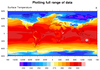
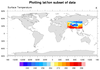
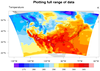
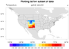
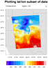
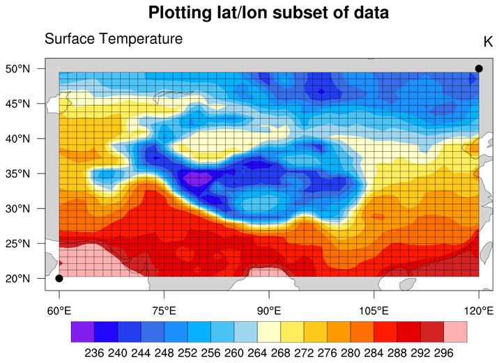
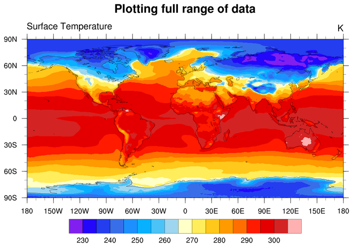
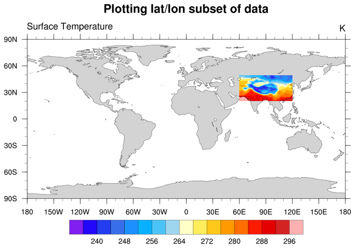
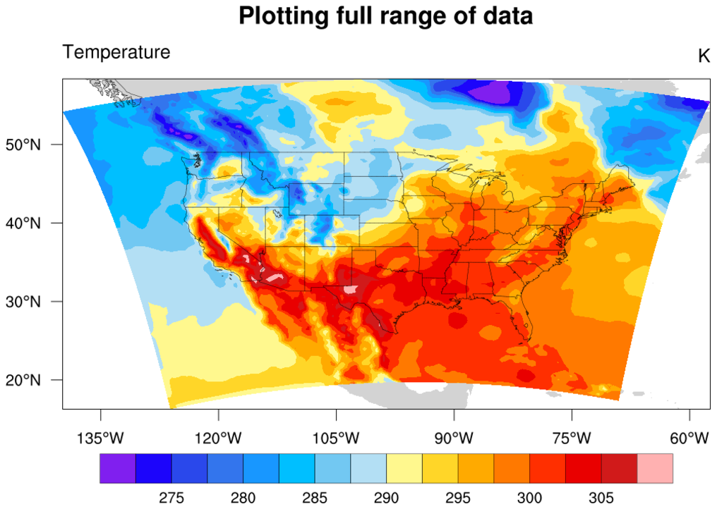
The first frame of this example shows the full global plot of the data. The second frame extracts a region in Asia using coordinate subscripting. The third frame zooms in on this region and adds a lat/lon grid and markers to further show the region of interest. The gsn_coordinates procedure is used to add the lat/lon grid lines. The fourth frame shows how to subscript the data using negative longitudes, after flipping it.

latlon_subset_2.ncl:

Data on a curvilinear grid, which is data represented by 2D lat/lon arrays, cannot be extracted using "coordinate scripting" mentioned in the first example on this page.

To find out if your data is on a curvilinear lat/lon grid, first try using printVarSummary to print information about the variable. Check if there is an attribute called "coordinates" (not to be confused with the "Coordinates:" section):

Variable: temp
Type: float
Total Size: 15120 bytes
            3780 values
Number of Dimensions: 3
Dimensions and sizes:[lv_SPDY3 | 6] x [gridx_236 | 30] x [gridy_236 | 21]
Coordinates:
Number Of Attributes: 13
. . .
long_name : Temperature
units : degK
_FillValue : 1e+20
coordinates : gridlat_236 gridlon_236

"temp" doesn't have any information in the "Coordinates:" section, so this tells you right away this data is NOT on a rectilinear grid. However, it does have an attribute called "coordinates", which tells you that this variable is represented by latitude and longitude arrays called "gridlat_236" and "gridlon_236". You can look on the same file that you read "temp" from, to see if these two variables are on the file.

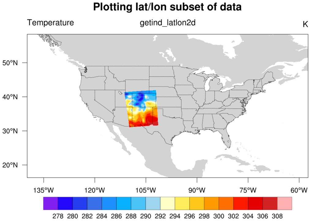
To extract a lat/lon region from curvilinear data, use the getind_latlon2d function. Assuming you have a 2D array "temp" with 2D lat/lon arrays that you've read off the file and named "lat2d", "lon2d":

  lat_pts  = (/30,60/)
  lon_pts  = (/ 0,50/)
  ij       = getind_latlon2d(lat2d,lon2d,lat_pts,lon_pts)
  temp_sub = temp(ij(0,0):ij(1,0),ij(0,1):ij(1,1))

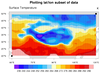
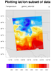
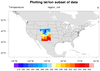
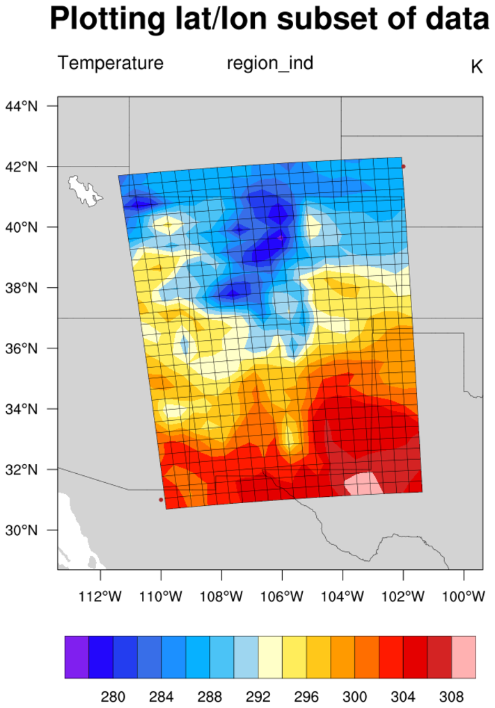
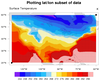
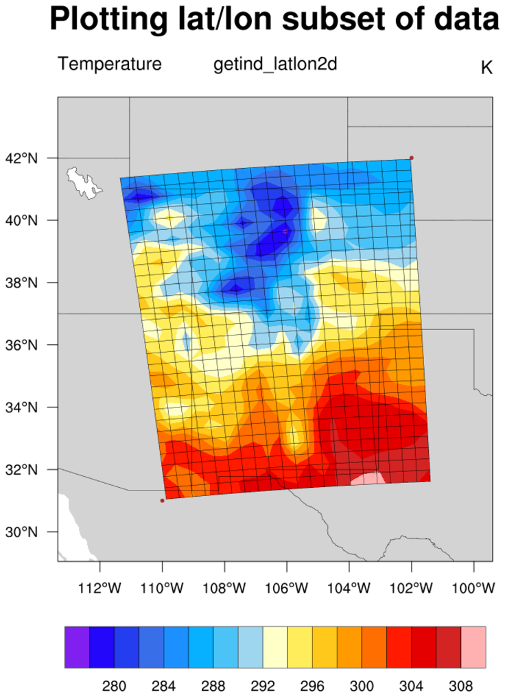
The first frame of this example shows the plot of the whole data array, which is regional data that covers the United States. The second frame extracts a region over New Mexico and Colorado using getind_latlon2d. The third frame zooms in on this region and adds a lat/lon grid and markers to further show the region of interest. The gsn_coordinates procedure is used to add the lat/lon grid lines.

See latlon_subset_3.ncl for an example of using region_ind. See latlon_subset_compare_3.ncl for a comparison of both methods.

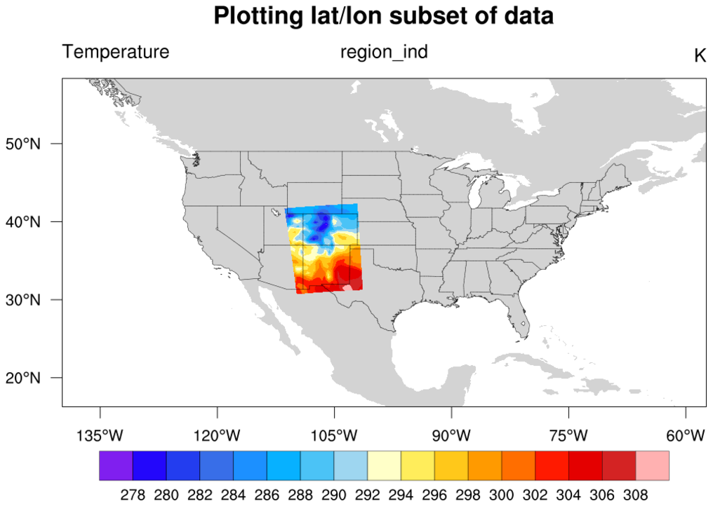
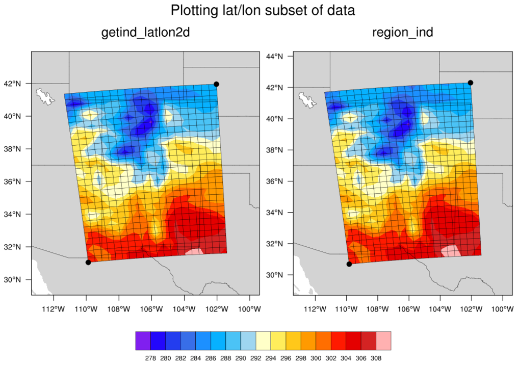
latlon_subset_3.ncl:

This example is exactly the same as latlon_subset_2 except the region_ind function is used.

What is the difference between the two functions? The getind_latlon2d uses arguments which specify two opposite corners of the region while region_ind's arguments specify the southern- (latS), northern- (latN), western- (latW) and eastern- (latE) most locations.

Clearly, when applied to the data of this example, the grid area difference is small. Different curvilinear grids may result in larger areal differences.

See latlon_subset_2.ncl for an example of using getind_latlon2d. See latlon_subset_compare_3.ncl for a comparison of both methods.

latlon_subset_compare_3.ncl:

This example is a panel plot of the third images from the previous two examples, allowing you to more easily compare the difference between the getind_latlon2d and region_ind functions.

Note that the lat/lon area created by using the region_ind function is slightly larger than the area created by the getind_latlon2d function.

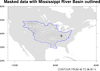
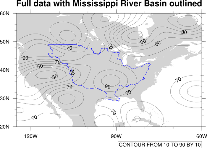
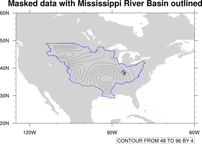
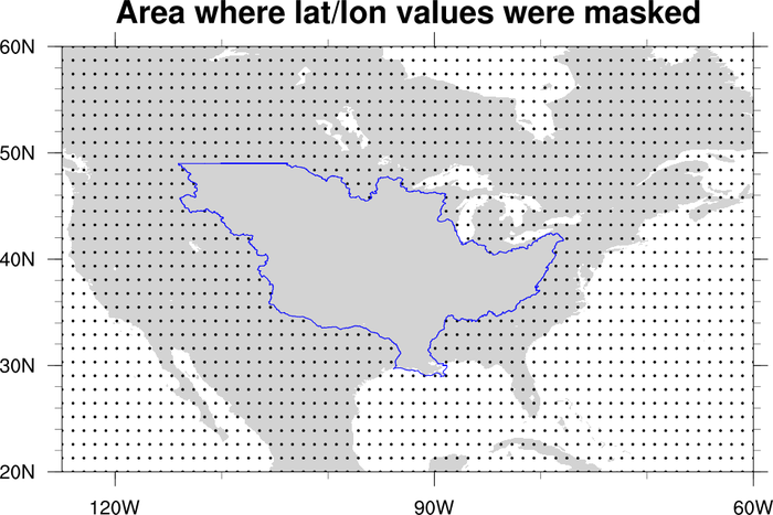
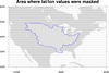mask_9.ncl: Demonstrates using gc_inout to mask an area in your data array using a geographical outline.

This particular example reads a shapefile to get an outline of the Mississippi River Basin. You then have the option of masking out all areas inside or outside this outline.

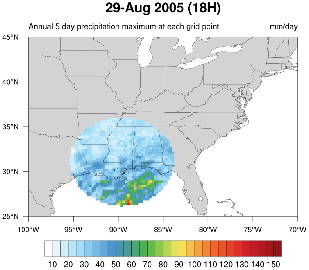
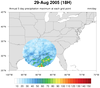Katrina_circle.ncl: This script plots the 5-day running average of precipitation for an entire year (2005). It shows a unique way of displaying filled contours in a circle, by using nggcog in conjunction with gc_inout to mask data inside a great circle.

See the Unique examples page for another version of this script that generates a histogram of the values, and for an animation of both scripts.

This code was contributed by Jake Huff, a Masters student in the Climate Extremes Modeling Group at Stony Brook University.

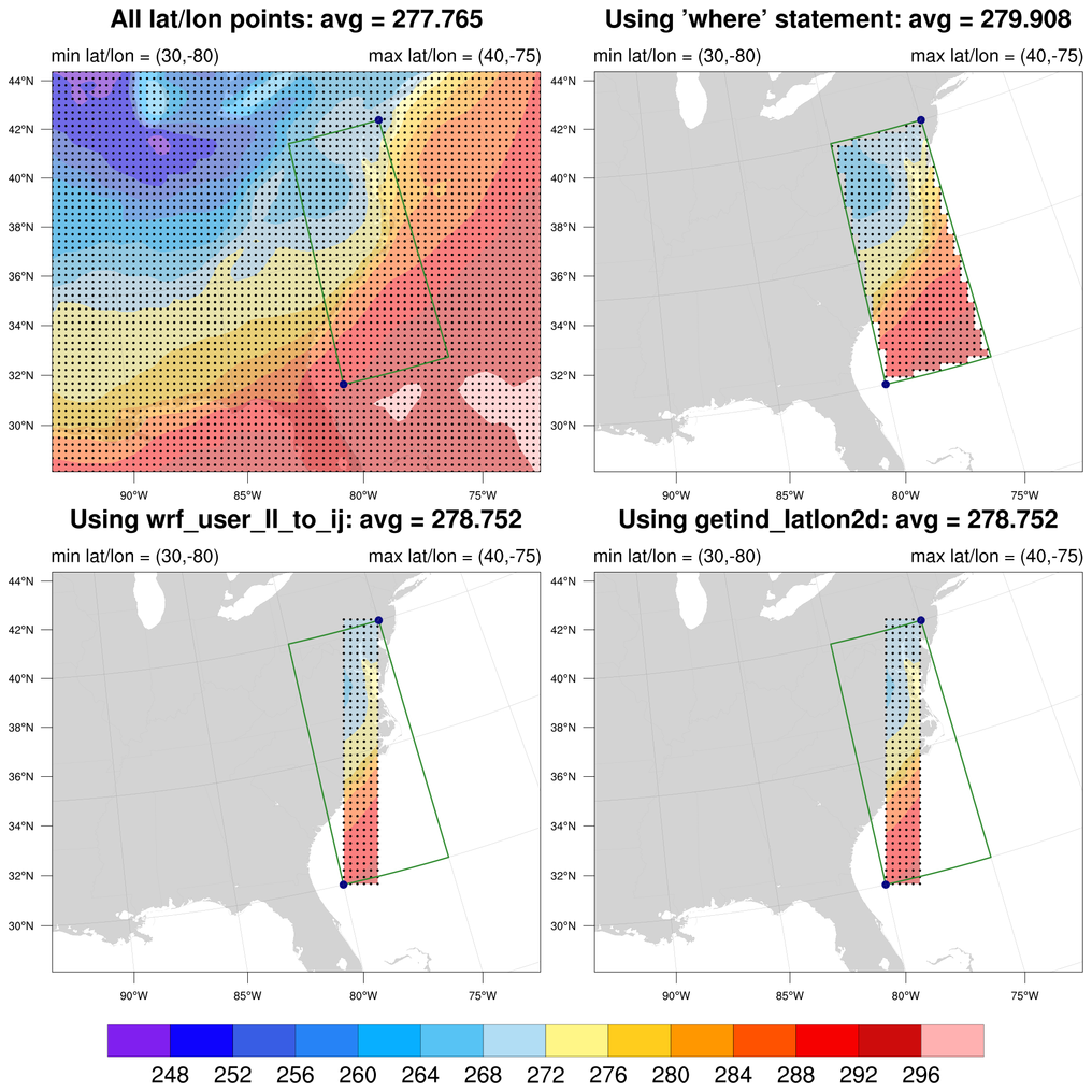
wrf_gsn_10.ncl This example shows three ways to subset a WRF lat/lon grid by providing two corners of a lat/lon box. Using each method, a spatial average is taken of the data in this box.

The three methods are 1) where, 2) wrf_user_ll_to_xy, 3) getind_latlon2d.

Markers are drawn in the plots to show the area where the data was subsetted, so you can see there is quite a difference in the two methods.

wrf_user_ll_to_xy should only be used on WRF-ARW data. The other methods will work on curvilinear grids.