NCL Home>
Application examples>
Data sets ||
Data files for some examples
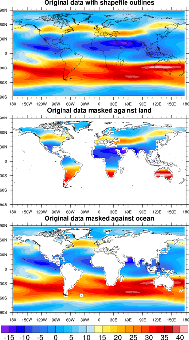
 shapefiles_1.ncl:
Demonstrates how to read a shapefile and draw filled polygons over a map.
Non-spatial variables from the associated database (i.e., the states.dbf
file) are used to compute the polygon colors.
shapefiles_1.ncl:
Demonstrates how to read a shapefile and draw filled polygons over a map.
Non-spatial variables from the associated database (i.e., the states.dbf
file) are used to compute the polygon colors.
 shapefiles_2.ncl:
Demonstrates how to read a shapefile and draw selected information
based upon a database query.
In this case, the historical incidents of F5-class tornadoes in
the USA are plotted.
shapefiles_2.ncl:
Demonstrates how to read a shapefile and draw selected information
based upon a database query.
In this case, the historical incidents of F5-class tornadoes in
the USA are plotted.
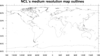
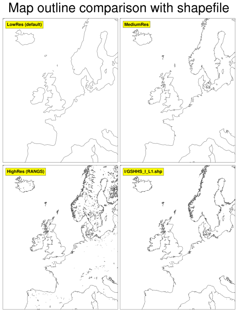
 mapoutlines_5.ncl:
This script demonstrates the difference in resolution between the
low resolution and medium resolution map databases of NCL,
and a world shapefile downloaded from
http://www.ngdc.noaa.gov/mgg/shorelines/data/gshhg/latest/.
mapoutlines_5.ncl:
This script demonstrates the difference in resolution between the
low resolution and medium resolution map databases of NCL,
and a world shapefile downloaded from
http://www.ngdc.noaa.gov/mgg/shorelines/data/gshhg/latest/.
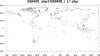
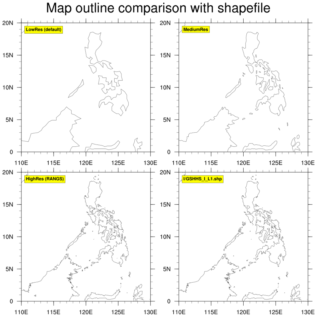
 mapoutlines_5_zoom.ncl:
This script is similar to the mapoutlines_5.ncl one above, except it
includes the "HighRes"
database, if installed. It produces two panel plots, so you can
compare the various map outlines.
mapoutlines_5_zoom.ncl:
This script is similar to the mapoutlines_5.ncl one above, except it
includes the "HighRes"
database, if installed. It produces two panel plots, so you can
compare the various map outlines.
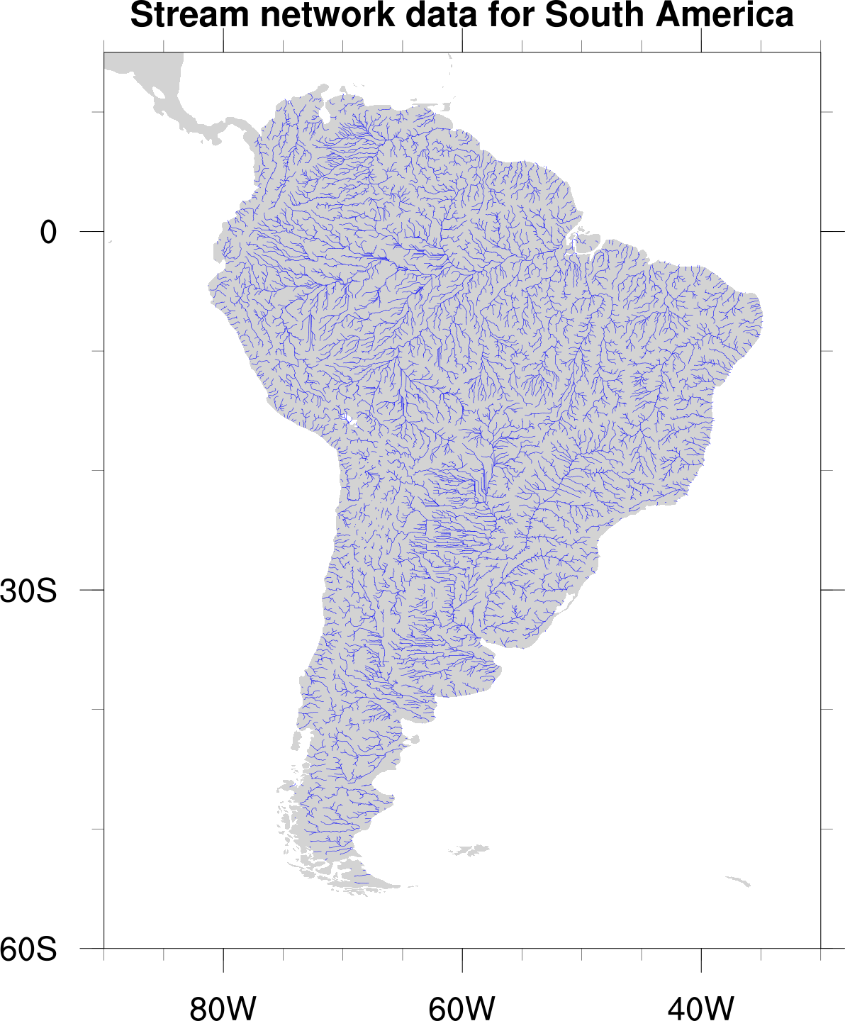
 shapefiles_3.ncl:
Demonstrates how to add shapefile outlines representing stream data in
South America to an NCL map using
gsn_add_shapefile_polylines.
shapefiles_3.ncl:
Demonstrates how to add shapefile outlines representing stream data in
South America to an NCL map using
gsn_add_shapefile_polylines.
 shapefiles_4.ncl: Demonstrates
using "shapefile_mask_data" to mask an area in your data array
using a geographical outline. This script
requires shapefile_utils.ncl.
shapefiles_4.ncl: Demonstrates
using "shapefile_mask_data" to mask an area in your data array
using a geographical outline. This script
requires shapefile_utils.ncl.
 shapefiles_5.ncl:
Makes use of several shapefiles of differing resolutions and contents to mask data along county borders (Pakistan), and to draw and label selected boundaries and cities. Demonstrates querying the shapefiles' databases via non-spatial attributes to extract and draw specific geometry.
shapefiles_5.ncl:
Makes use of several shapefiles of differing resolutions and contents to mask data along county borders (Pakistan), and to draw and label selected boundaries and cities. Demonstrates querying the shapefiles' databases via non-spatial attributes to extract and draw specific geometry.
 shapefiles_6.ncl:
This example uses a script very similar to example 3 above for South
America to draw the canton outlines for Switzerland. The first frame
shows the default map outline for Switzerland (admittedly not very good),
and the second frame shows the data from the shapefile.
shapefiles_6.ncl:
This example uses a script very similar to example 3 above for South
America to draw the canton outlines for Switzerland. The first frame
shows the default map outline for Switzerland (admittedly not very good),
and the second frame shows the data from the shapefile.
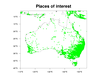
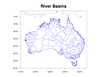 shapefiles_7.ncl:
This script uses several shapefiles to draw river basins, points of
interest, and indigenous areas in Australia. The shapefiles were
downloaded from several locations. See the comments in
the script for details.
shapefiles_7.ncl:
This script uses several shapefiles to draw river basins, points of
interest, and indigenous areas in Australia. The shapefiles were
downloaded from several locations. See the comments in
the script for details.
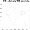
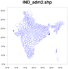
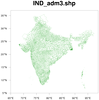
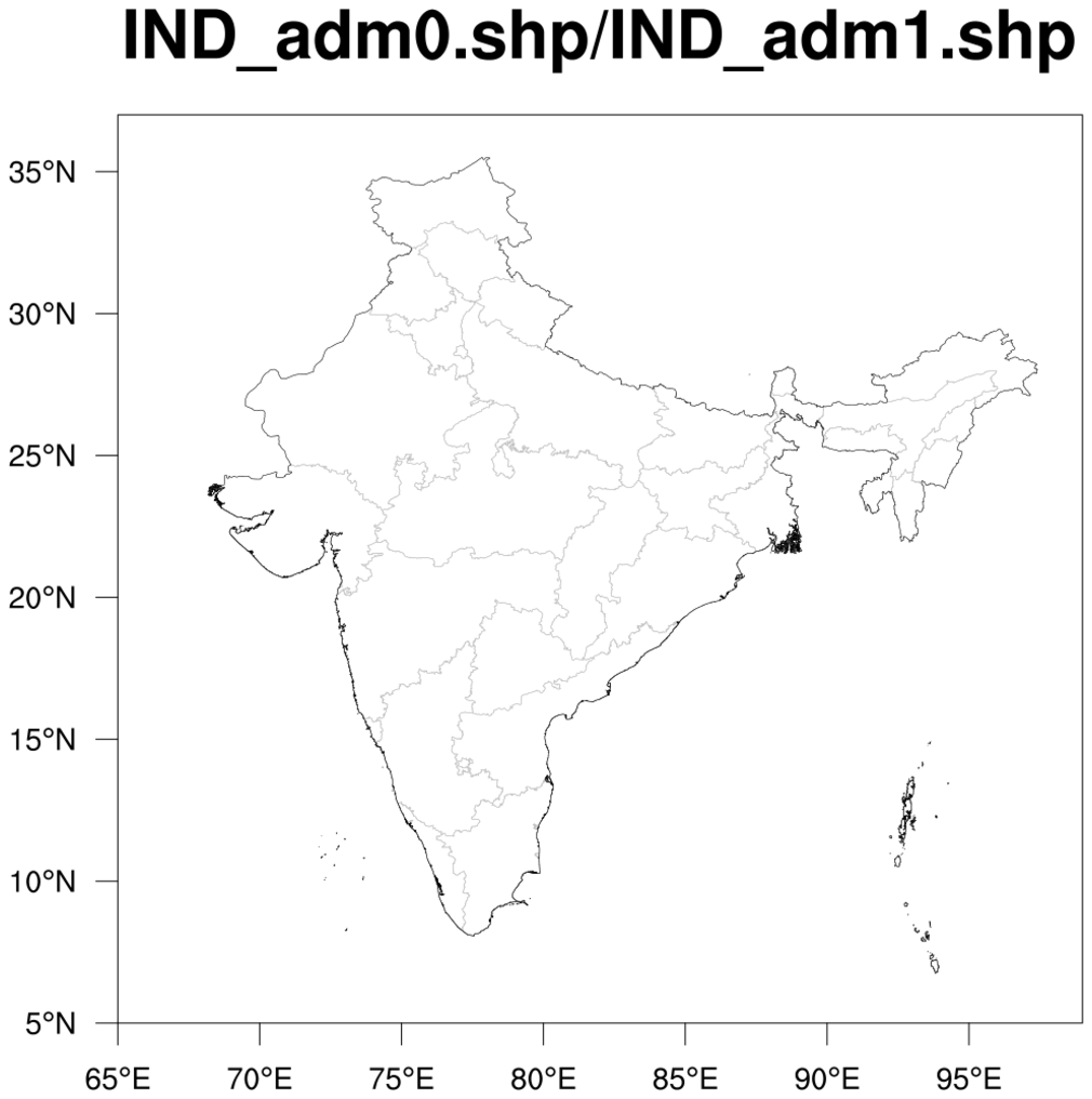
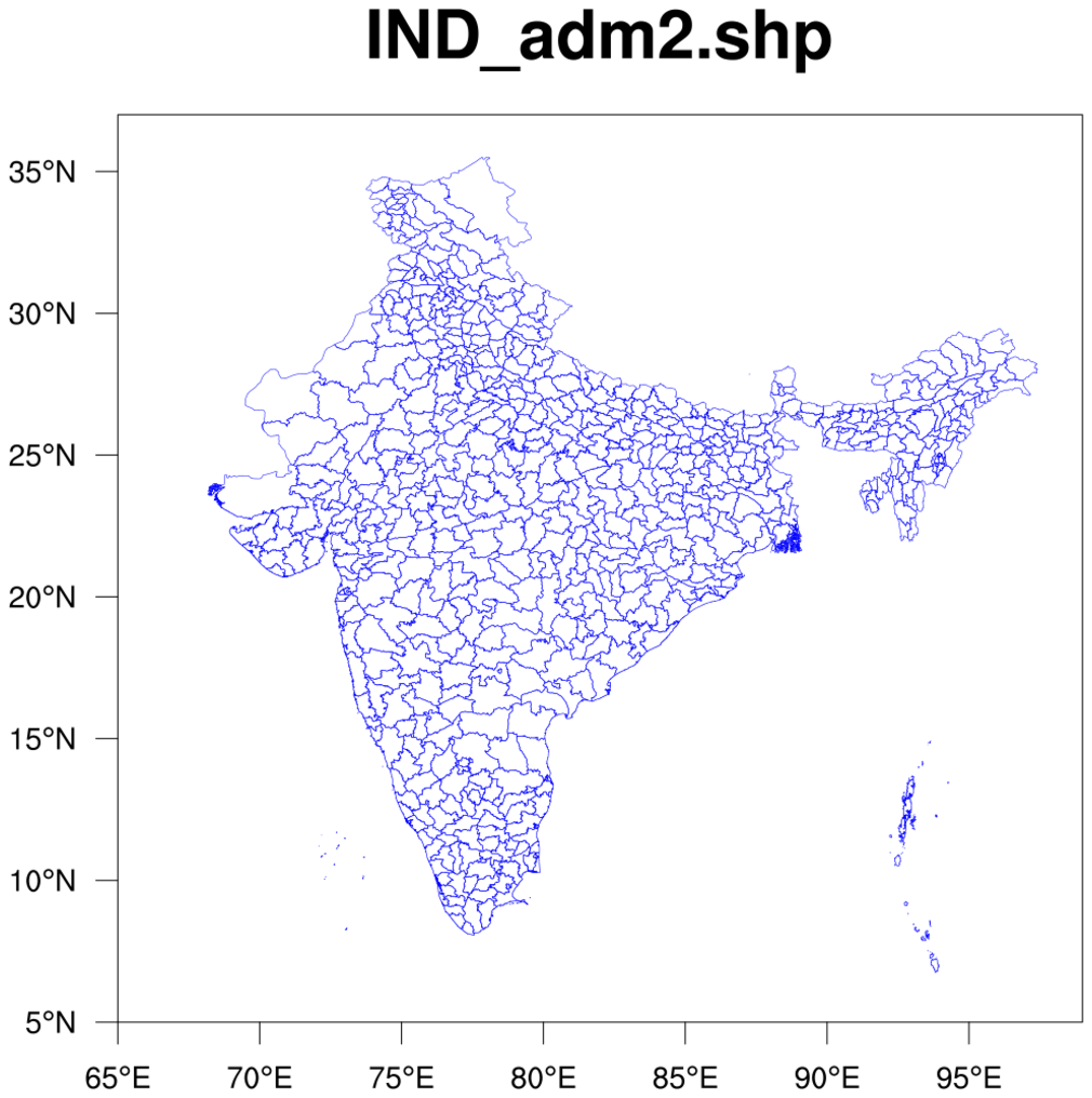
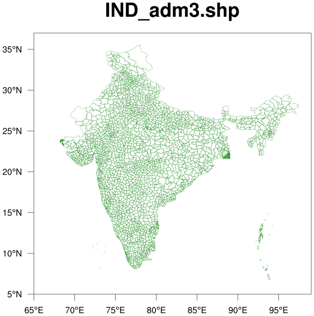
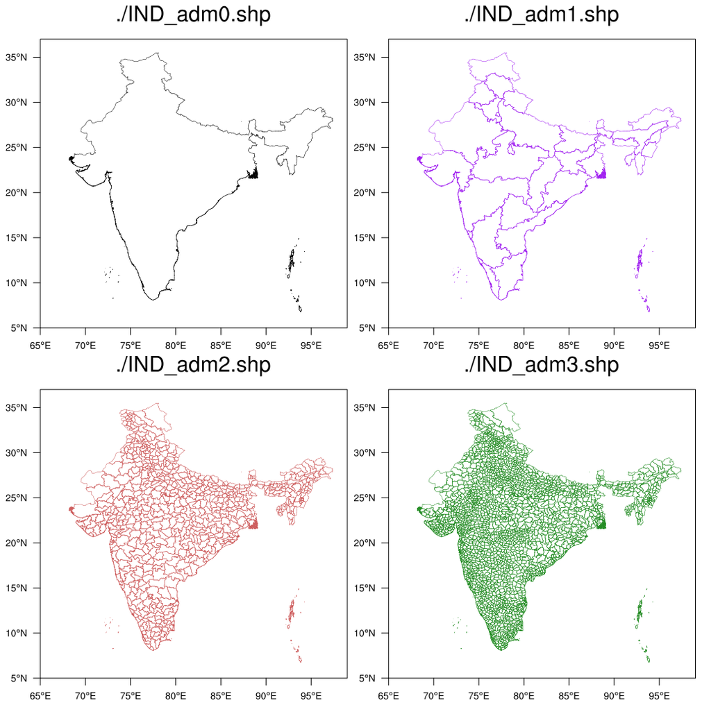
 shapefiles_8.ncl /
shapefiles_8_panel.ncl:
This script uses four shapefiles downloaded from
http://www.gadm.org/country
to draw various administrative areas for India.
shapefiles_8.ncl /
shapefiles_8_panel.ncl:
This script uses four shapefiles downloaded from
http://www.gadm.org/country
to draw various administrative areas for India.
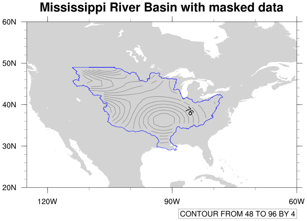
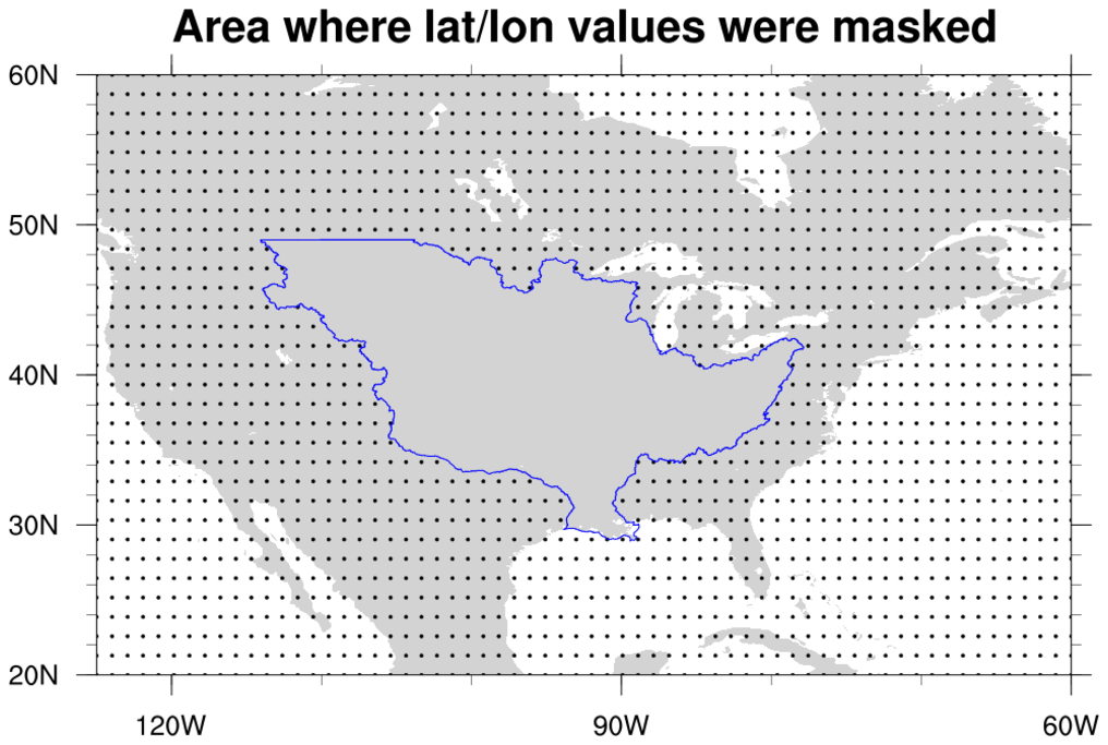
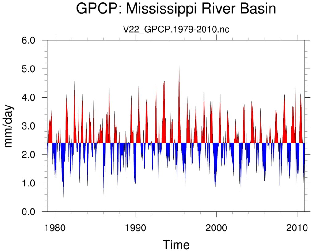
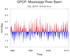 shapefiles_9.ncl:
This uses the shapefile Example 4.
This demonstrates calculating an areally weighted mean time series
for an irregularly shaped region. As in Example 4, an array containing
only the desired locations inside the shapefile is created. All other
grid points are set to _FillValue. Specifially, this computes the
areal mean time series of monthly precipitation for the Mississippi
River Basin. The data is the monthly GPCP.
shapefiles_9.ncl:
This uses the shapefile Example 4.
This demonstrates calculating an areally weighted mean time series
for an irregularly shaped region. As in Example 4, an array containing
only the desired locations inside the shapefile is created. All other
grid points are set to _FillValue. Specifially, this computes the
areal mean time series of monthly precipitation for the Mississippi
River Basin. The data is the monthly GPCP.
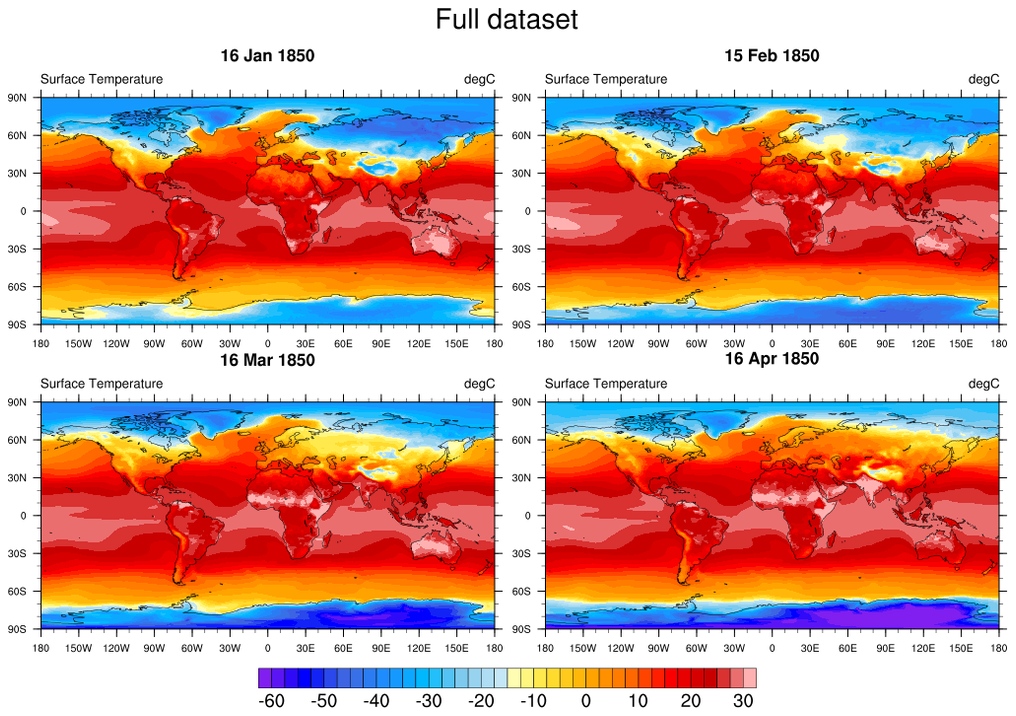
 mask_12.ncl: This example shows how
to use a shapefile that contains polygon outlines to create a data
mask for a variable with 1D coordinate arrays. The mask array is then
written to a copy of the input file. [This script
requires shapefile_utils.ncl.]
mask_12.ncl: This example shows how
to use a shapefile that contains polygon outlines to create a data
mask for a variable with 1D coordinate arrays. The mask array is then
written to a copy of the input file. [This script
requires shapefile_utils.ncl.]
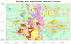

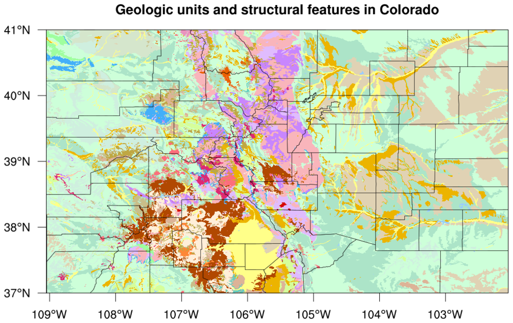
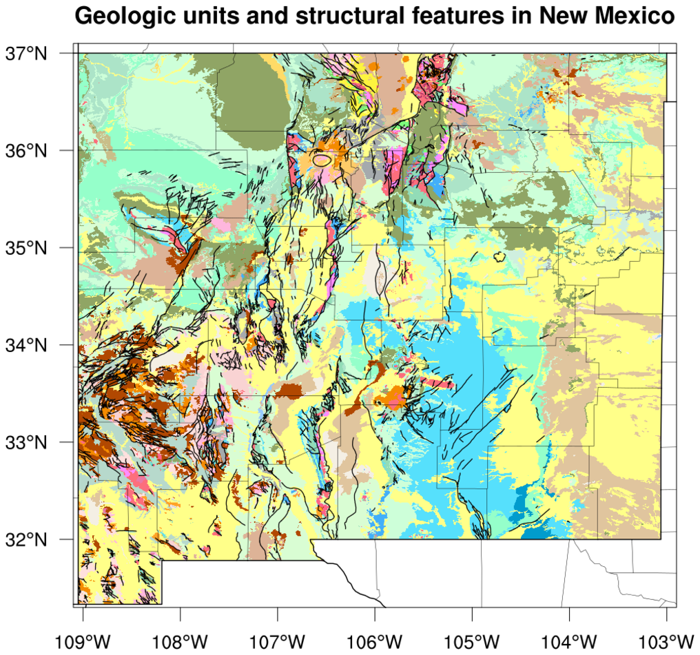
 shapefiles_10.ncl /
shapefiles_NM_10.ncl: These
examples show how to plot polygon data from a shapefile containing
geologic units and structural features in Colorado and New Mexico. The shapefiles were
downloaded from
http://mrdata.usgs.gov/geology/state/.
shapefiles_10.ncl /
shapefiles_NM_10.ncl: These
examples show how to plot polygon data from a shapefile containing
geologic units and structural features in Colorado and New Mexico. The shapefiles were
downloaded from
http://mrdata.usgs.gov/geology/state/.
 shapefiles_11.ncl: This
example shows how to use a shapefile that contains an outline of the
United States to create a land mask. The land mask is written to a
NetCDF file so you can use it later for masking other variables on the
same grid.
shapefiles_11.ncl: This
example shows how to use a shapefile that contains an outline of the
United States to create a land mask. The land mask is written to a
NetCDF file so you can use it later for masking other variables on the
same grid.
 shapefiles_12.ncl /
shapefiles_12b.ncl: This
example shows how to
modify gsn_add_shapefile_polylines
to have it draw only a subset of the features in the given shapefile.
shapefiles_12.ncl /
shapefiles_12b.ncl: This
example shows how to
modify gsn_add_shapefile_polylines
to have it draw only a subset of the features in the given shapefile.
 shapefiles_13.ncl: This
example shows how to use shapefile data to collect lat/lon data points
in each county of Georgia, and take an average of all the data values
in that county. Based on each county average, a fill color is assigned
and the county is filled using
modify gsn_add_polygon.
shapefiles_13.ncl: This
example shows how to use shapefile data to collect lat/lon data points
in each county of Georgia, and take an average of all the data values
in that county. Based on each county average, a fill color is assigned
and the county is filled using
modify gsn_add_polygon.
 shapefiles_14.ncl: This
example shows how to add shapefile outlines to an existing WRF
contour/map plot.
shapefiles_14.ncl: This
example shows how to add shapefile outlines to an existing WRF
contour/map plot.
 shapefiles_14_mask.ncl: This
example is similar to the previous one, except it masks the WRF "hgt"
variable against a select list of U.S. states outlines from the
shapefile.
shapefiles_14_mask.ncl: This
example is similar to the previous one, except it masks the WRF "hgt"
variable against a select list of U.S. states outlines from the
shapefile.
 Germany_coastal_counties_DEU_adm.ncl:
This script, contributed by Karin Meier-Fleischer
of Deutsche Klimarechenzentrum
(DKRZ), shows how to use the DEU_adm3.shp shapefile downloaded
from http://www.gadm.org/country
to average data over coastal counties of Germany.
Germany_coastal_counties_DEU_adm.ncl:
This script, contributed by Karin Meier-Fleischer
of Deutsche Klimarechenzentrum
(DKRZ), shows how to use the DEU_adm3.shp shapefile downloaded
from http://www.gadm.org/country
to average data over coastal counties of Germany.

 France_1.ncl /
France_2.ncl /
France_3.ncl:
The purpose of this example is to demonstrate the use of the
gsSegments and
gsColors
resources added in
added in version 6.2.0,
and how much routines like
gsn_add_shapefile_polygons,
gsn_add_shapefile_polylines,
gsn_add_polyline,
gsn_add_polygon
have been sped-up
in version 6.2.0.
France_1.ncl /
France_2.ncl /
France_3.ncl:
The purpose of this example is to demonstrate the use of the
gsSegments and
gsColors
resources added in
added in version 6.2.0,
and how much routines like
gsn_add_shapefile_polygons,
gsn_add_shapefile_polylines,
gsn_add_polyline,
gsn_add_polygon
have been sped-up
in version 6.2.0.
 shapefiles_15.ncl: This
example is another one showing the difference between map outlines in
NCL and map outlines added from a shapefile. The first plot in the
panel shows the counties of Colorado as plotted from NCL, and the
second plot shows the counties as plotted from the USA_adm2 shapefile
downloaded from
http://www.gadm.org/country.
shapefiles_15.ncl: This
example is another one showing the difference between map outlines in
NCL and map outlines added from a shapefile. The first plot in the
panel shows the counties of Colorado as plotted from NCL, and the
second plot shows the counties as plotted from the USA_adm2 shapefile
downloaded from
http://www.gadm.org/country.
 shapefiles_16.ncl: This
example shows the effect that shapefile masking will have on both a
coarse (32 x 64) and fine (64 x 128) grid.
shapefiles_16.ncl: This
example shows the effect that shapefile masking will have on both a
coarse (32 x 64) and fine (64 x 128) grid.
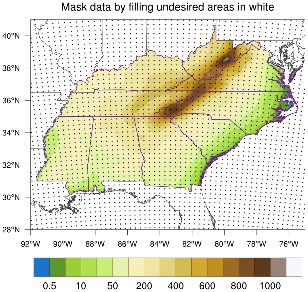
 shapefiles_17.ncl: This
example shows two ways to mask data based out outlines in a
shapefile: one is to use the shapefile_mask_data function
mentioned in previous examples, and another is to simply fill
in the undesired outlines in white over the original
contour data, effectively masking it.
shapefiles_17.ncl: This
example shows two ways to mask data based out outlines in a
shapefile: one is to use the shapefile_mask_data function
mentioned in previous examples, and another is to simply fill
in the undesired outlines in white over the original
contour data, effectively masking it.
 shapefiles_18.ncl: This
example uses a modified version of "shapefile_mask_data" to
mask data based on a shapefile outline, and a "delta" distance
(in km) outside the shapefile outline. See "delta_kilometer"
in the script.
shapefiles_18.ncl: This
example uses a modified version of "shapefile_mask_data" to
mask data based on a shapefile outline, and a "delta" distance
(in km) outside the shapefile outline. See "delta_kilometer"
in the script.
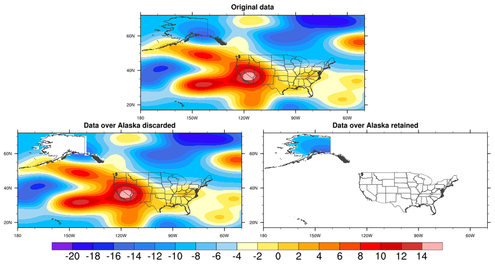
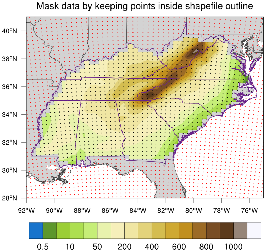
 shapefiles_19.ncl:
This example shows how to either mask (retain) or remove data, based on a shapefile
outline. We get a lot of questions on this topic, so we decided to create a very
basic example that shows both types of masking.
shapefiles_19.ncl:
This example shows how to either mask (retain) or remove data, based on a shapefile
outline. We get a lot of questions on this topic, so we decided to create a very
basic example that shows both types of masking.
 shapefiles_20.ncl:
This example shows how to use the shapefile_mask_data function in
shapefile_utils.ncl
to return a mask array, and then apply this mask array to a variable
with multiple time steps. The special option "return_mask" is
set to True, telling the function to return the 0/1 mask array,
instead of returning the masked data itself.
shapefiles_20.ncl:
This example shows how to use the shapefile_mask_data function in
shapefile_utils.ncl
to return a mask array, and then apply this mask array to a variable
with multiple time steps. The special option "return_mask" is
set to True, telling the function to return the 0/1 mask array,
instead of returning the masked data itself.
 shapefiles_21.ncl:
This example demonstrates two ways to mask data based on shapefile
outlines of interest.
shapefiles_21.ncl:
This example demonstrates two ways to mask data based on shapefile
outlines of interest.

 shapefiles_22.ncl: This
example shows how to use two different shapefiles to mask data. One
shapefile contains a single outline of the Caspian Sea, and the other
contains outlines of isles inside the Caspian Sea.
shapefiles_22.ncl: This
example shows how to use two different shapefiles to mask data. One
shapefile contains a single outline of the Caspian Sea, and the other
contains outlines of isles inside the Caspian Sea.
 shapefiles_23.ncl: This script
shows how to use shapefile_mask_data to create a mask array for
masking a WRF output variable against an outline in a shapefile. It
then uses this mask array to mask select variables on the file.
shapefiles_23.ncl: This script
shows how to use shapefile_mask_data to create a mask array for
masking a WRF output variable against an outline in a shapefile. It
then uses this mask array to mask select variables on the file.
 shapefiles_24.ncl: This script
uses a shapefile outline to mask some data, and then calculates the
approximate area (in km^2) of the valid data that was retained
inside the shapefile area.
shapefiles_24.ncl: This script
uses a shapefile outline to mask some data, and then calculates the
approximate area (in km^2) of the valid data that was retained
inside the shapefile area.
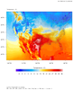
 shapefiles_25.ncl:
Read hourly METAR precipitation values for August 2018 at station locations.
Calculate monthly total precipitation at each station. Use Barnes iterative
correction (obj_anl_ic) to regrid the
data onto a user defined grid. Use a shape file to create grid mask to eliminate
values outside the coterminus USA. Plot as 'raster' to illustrate the underlying
grid resolution.
shapefiles_25.ncl:
Read hourly METAR precipitation values for August 2018 at station locations.
Calculate monthly total precipitation at each station. Use Barnes iterative
correction (obj_anl_ic) to regrid the
data onto a user defined grid. Use a shape file to create grid mask to eliminate
values outside the coterminus USA. Plot as 'raster' to illustrate the underlying
grid resolution.
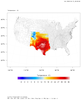
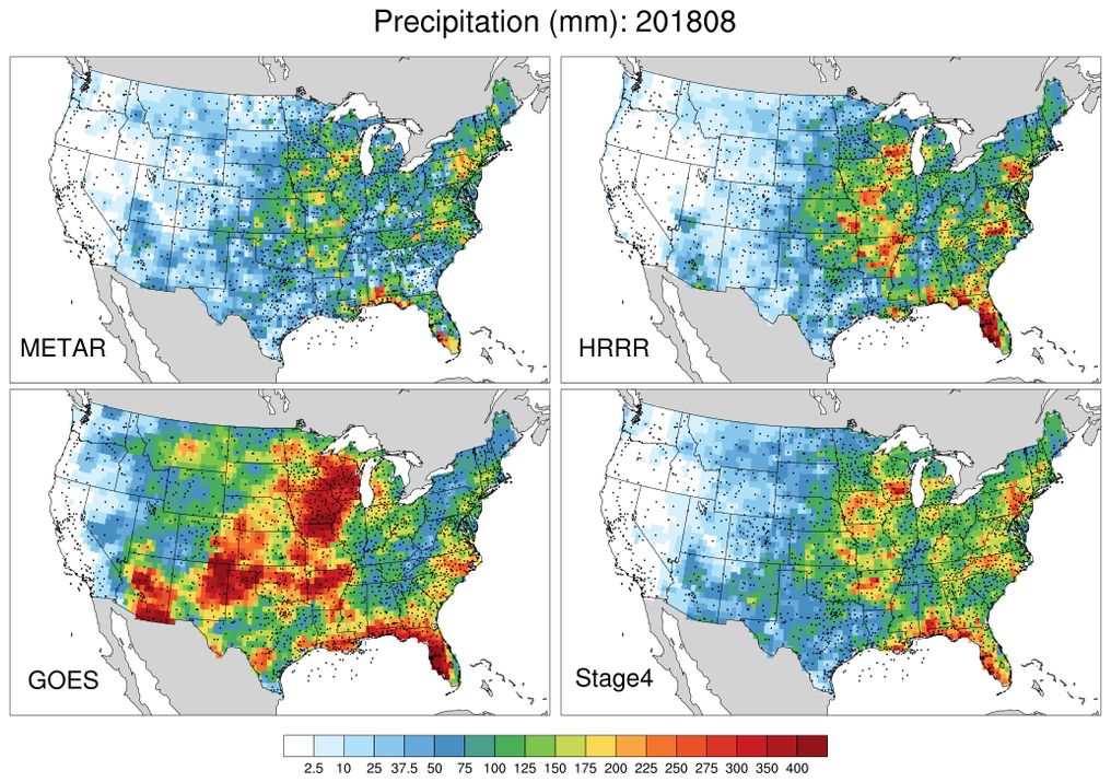
 shapefiles_26.ncl:
Similar to shapefiles_25 except values from four different sources
(METAR, HRR, GOES, Stage4) are used. The mask file created and saved
in shapefiles_25 is used to mask values outside the coterminus USA.
Plot as a panel.
shapefiles_26.ncl:
Similar to shapefiles_25 except values from four different sources
(METAR, HRR, GOES, Stage4) are used. The mask file created and saved
in shapefiles_25 is used to mask values outside the coterminus USA.
Plot as a panel.
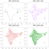
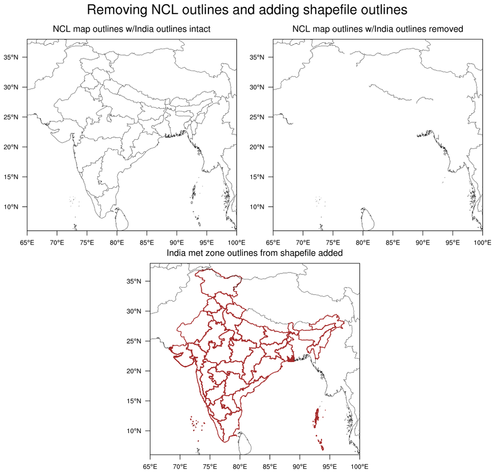
 maponly_30.ncl: This script
shows how to use the mpMaskOutlineSpecifiers
to remove the outlines of India, while keeping outlines from surrounding
countries. In the third plot, meteorological subdivisions of India
were added using a shapefile downloaded off the web.
maponly_30.ncl: This script
shows how to use the mpMaskOutlineSpecifiers
to remove the outlines of India, while keeping outlines from surrounding
countries. In the third plot, meteorological subdivisions of India
were added using a shapefile downloaded off the web.
Example pages containing:
tips |
resources |
functions/procedures
NCL: Plotting and working with shapefiles
Webinar: NCL and Shapefiles
Shapefiles
Shapefiles are a
From Wikipedia:
The Esri* Shapefile or simply
a shapefile is a popular geospatial vector data format for
geographic information systems software. It is developed and regulated
by Esri as a (mostly) open specification for data interoperability
among ESRI and other software products.[1] A "shapefile" commonly
refers to a collection of files with ".shp", ".shx", ".prj", ".dbf",
and other extensions on a common prefix name (e.g., "lakes.*"). The
actual shapefile relates specifically to files with the ".shp"
extension, however this file alone is incomplete for distribution, as
these other supporting files are required.
*Esri and the Esri Logo are licensed trademarks of
Environmental Systems Research Institute, Inc.
Shapefiles describe a homogeneous set of geometrical features comprised of either points, polylines, or polygons. These, for example, could represent water wells, rivers, and lakes, respectively. Each feature may also have non-spatial attributes that describe it, such as the name or temperature.
The Global Administrative Database
(GADM) offers consistent administrative boundaries at multiple levels.
The level 0 database (nations) is good to use for global or mesoscale
results, level 1 is the first level of sub-national administration
(typically states/provinces and territories) while level 2 offers the
second level of administration and is potentially useful for
high-resolution plots. Sometimes there are more levels (for example,
France has 6) with even higher resolution. The global shapefiles are
large, but it's possible to download individual countries separately.
NOAA provides some useful AWIPS
shapefile data.
Shapefile plotting and masking routines
These functions can be used to draw polygons, lines, and markers from shapefile data:
The shapefile_utils.ncl script provides additional useful routines for working with shapefiles:
- print_shapefile_info - prints information about the shapefile
- plot_shapefile - creates a basic map plot with the shapefile outlines added
- shapefile_mask_data - masks your own data against outlines in a shapefile
Important note: The shapefile_mask_data function is a powerful function used by many scripts on this page. In order for your data to be masked correctly using this function, your longitude values must be in the same range as the longitude values on the shapefile. Most shapefile longitude values are in the range -180 to 180. You can use the print_shapefile_info procedure above to print this information.
For a sample of the first two routines, try this simple 4-line NCL script with your own shapefile data, or download sample shapefiles here.
load "./shapefile_utils.ncl"
sname = "states.shp"
print_shapefile_info(sname)
plot_shapefile(sname)
Shapefile details
What follows are details of the contents of a shapefile. Several functions (see above) have been added to hide some of this detail.
Within NCL, a shapefile appears as a collection of 4 or 5 specifically named variables that encode the geometry of the features, along with some number of non-spatial variables. The number, names and types of the non-spatial variables depend upon the specific shapefile. The geometry of a feature is composed of one or more segments. Segments in turn are composed of an ordered-list of X, Y (and optionally Z) tuples. NCL uses the following variables to encode these relationships:
    geometry(num_features, 2)
    segments(num_segments, 2)
    x(num_points)
    y(num_points)
    z(num_points)    ; 3D datasets only
Each feature in the shapefile is represented by an entry in the geometry variable, along with corresponding entries in the non-spatial variables; i.e., the data for the i-th feature is found at the i-th entry of these variables. Each entry in geometry has two values: geometry(i, 0) specifies the index into variable segments of the 1st segment of the i-th feature, and geometry(i, 1) denotes the number of segments that make up the feature.
Similarly, each entry in segments has two values: segments(j, 0) is the index of the 1st XY(Z) tuple of the j-th segment, and segments(j, 1) is the number of tuples belonging to the segment.
With this encoding, any subsequent segments belonging to the i-th feature follow its first one in segments, and all the XY(Z) tuples belonging to the j-th segment follow the first in the x,y,(z) variables.
NCL defines several global attributes for a shapefile:
    geom_segIndex = 0
    geom_numSegs  = 1
    segs_xyzIndex = 0
    segs_numPnts  = 1
    geometry_type = "point" | "polyline" | "polygon"
    layer_name    =    ; value derived from the shapefile
The first 4 attributes are intended as symbolic indices into the geometry and segments variable; see the examples below for how they should be used.
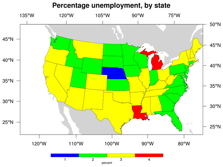
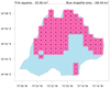
 shapefiles_1.ncl:
Demonstrates how to read a shapefile and draw filled polygons over a map.
Non-spatial variables from the associated database (i.e., the states.dbf
file) are used to compute the polygon colors.
shapefiles_1.ncl:
Demonstrates how to read a shapefile and draw filled polygons over a map.
Non-spatial variables from the associated database (i.e., the states.dbf
file) are used to compute the polygon colors.
To run this example, you must have the files "states.shp", "states.dbf", and "states.shx". These can be obtained from the National Map.
A Python version of this projection is available here.
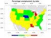
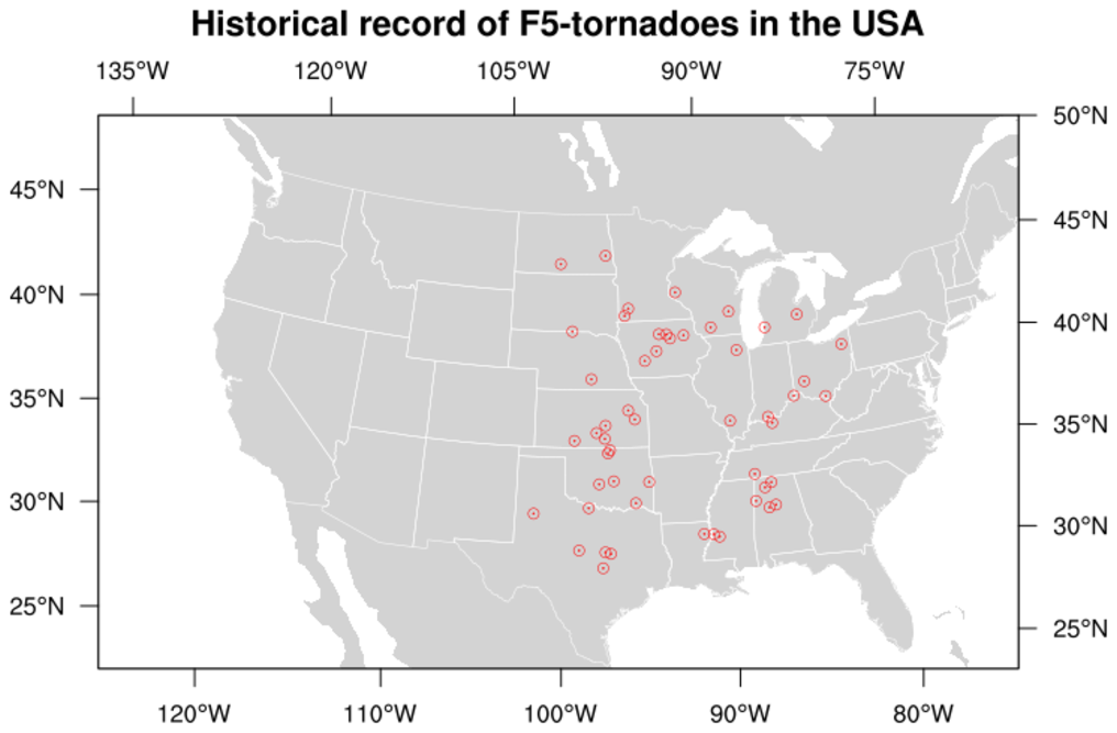 shapefiles_2.ncl:
Demonstrates how to read a shapefile and draw selected information
based upon a database query.
In this case, the historical incidents of F5-class tornadoes in
the USA are plotted.
shapefiles_2.ncl:
Demonstrates how to read a shapefile and draw selected information
based upon a database query.
In this case, the historical incidents of F5-class tornadoes in
the USA are plotted.
To run this example, you must have the "states" shapefiles from the previous example, along with "tornadx020.shp", "tornadx020.dbf", and "tornadx020.shx". These can be obtained from the USGS's holdings on data.gov.
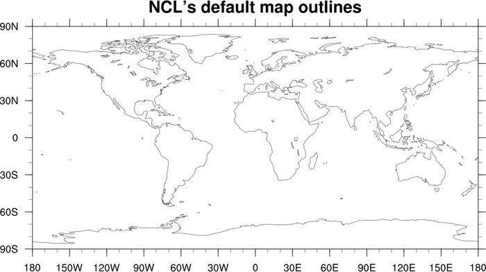
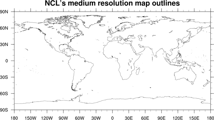
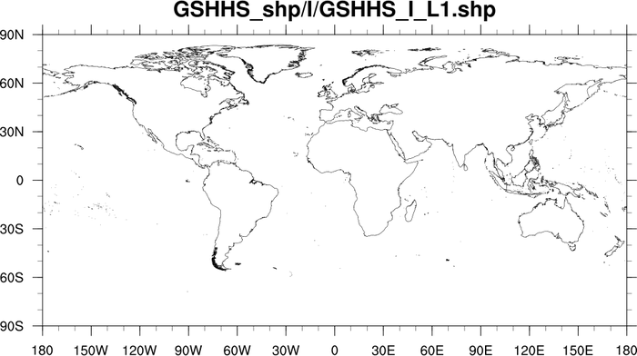 mapoutlines_5.ncl:
This script demonstrates the difference in resolution between the
low resolution and medium resolution map databases of NCL,
and a world shapefile downloaded from
http://www.ngdc.noaa.gov/mgg/shorelines/data/gshhg/latest/.
mapoutlines_5.ncl:
This script demonstrates the difference in resolution between the
low resolution and medium resolution map databases of NCL,
and a world shapefile downloaded from
http://www.ngdc.noaa.gov/mgg/shorelines/data/gshhg/latest/.
You cannot use the "HighRes" database with a global map, so the shapefile outlines are your best bet if you need more resolution.
 mapoutlines_5_zoom.ncl:
This script is similar to the mapoutlines_5.ncl one above, except it
includes the "HighRes"
database, if installed. It produces two panel plots, so you can
compare the various map outlines.
mapoutlines_5_zoom.ncl:
This script is similar to the mapoutlines_5.ncl one above, except it
includes the "HighRes"
database, if installed. It produces two panel plots, so you can
compare the various map outlines.
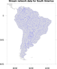
 shapefiles_3.ncl:
Demonstrates how to add shapefile outlines representing stream data in
South America to an NCL map using
gsn_add_shapefile_polylines.
shapefiles_3.ncl:
Demonstrates how to add shapefile outlines representing stream data in
South America to an NCL map using
gsn_add_shapefile_polylines.
To run this example, you must download the "HYDRO1k Streams data set
for South America as a tar file in shapefile format" (2.4 MB) from:
http://eros.usgs.gov/#/Find_Data/Products_and_Data_Available/gtopo30/hydro/samerica
Note: this dataset no longer appears to be available as of February 2014.
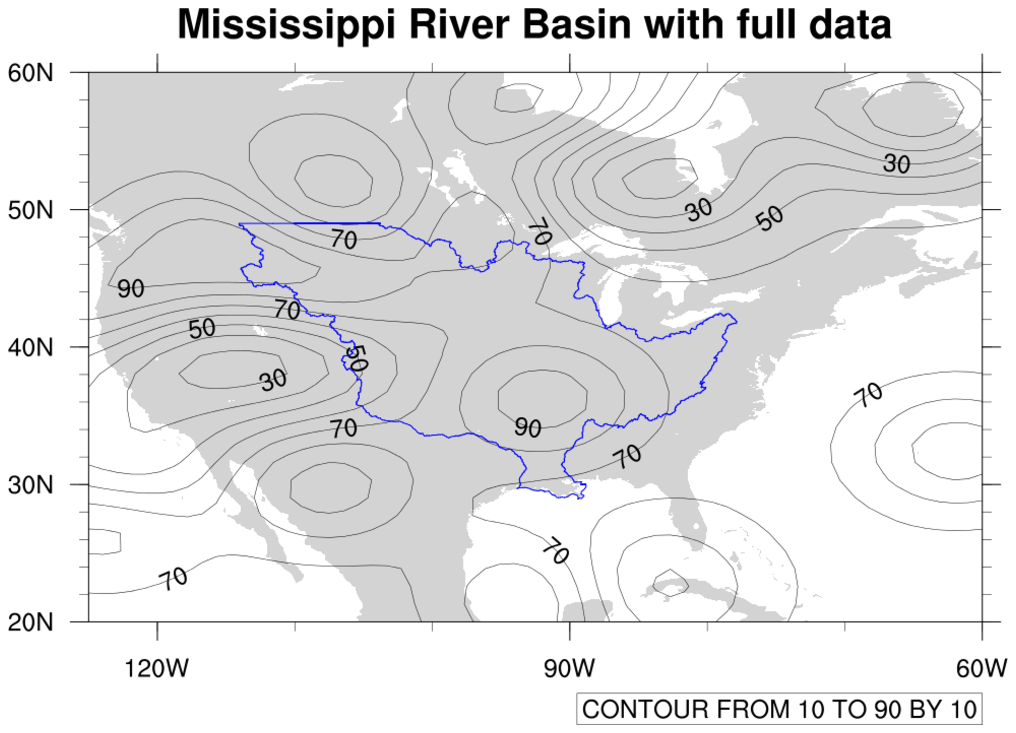
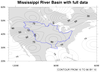
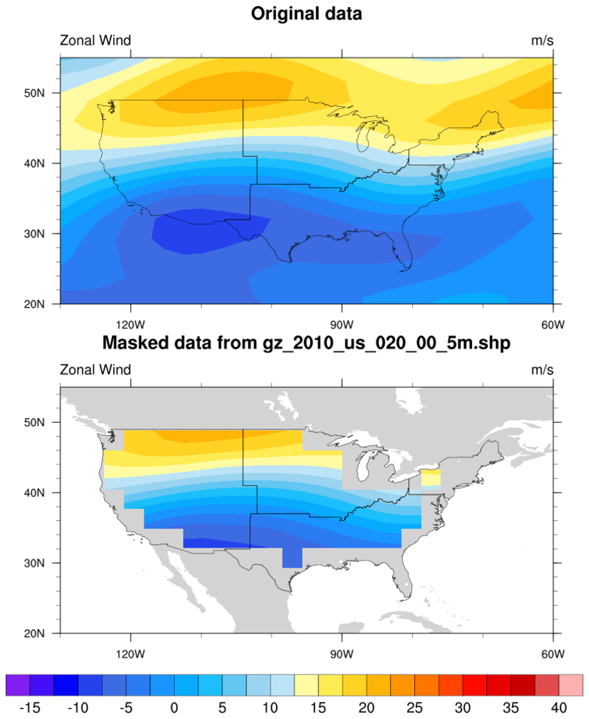
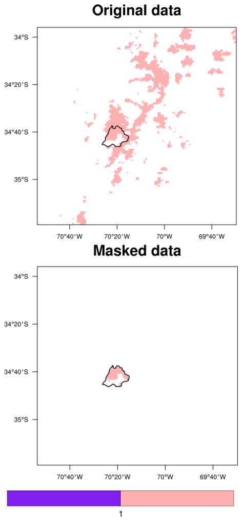
 shapefiles_4.ncl: Demonstrates
using "shapefile_mask_data" to mask an area in your data array
using a geographical outline. This script
requires shapefile_utils.ncl.
shapefiles_4.ncl: Demonstrates
using "shapefile_mask_data" to mask an area in your data array
using a geographical outline. This script
requires shapefile_utils.ncl.
See the description of this function for important information.
This particular example reads a shapefile to get an outline of the Mississippi River Basin. You then have the option of masking out all areas inside or outside this outline.
The "mrb.xxx" data files for this example can be found on the example datasets page.
The shapefiles_4_old.ncl is an older script that doesn't use a separate function to mask the data. Look at this script if you are interested in seeing the "guts" of what it takes to mask data against a shapefile outline.
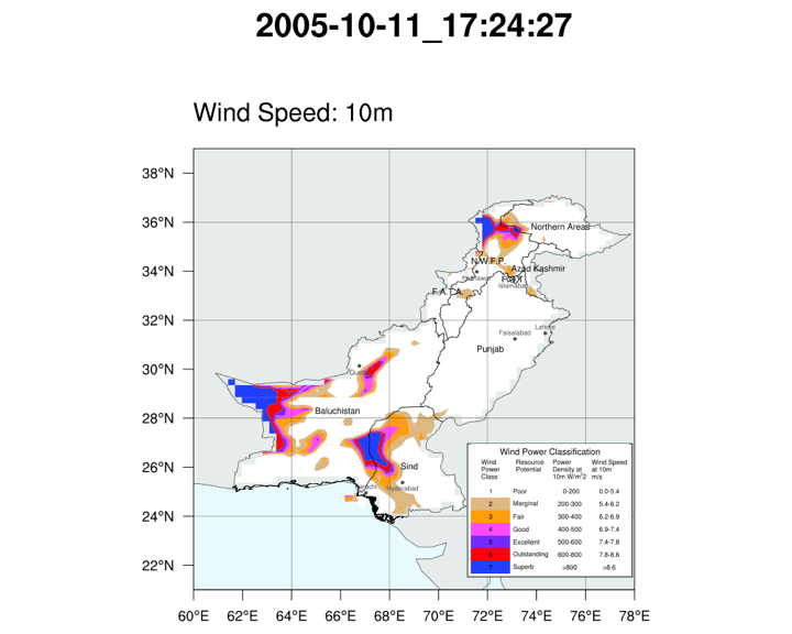 shapefiles_5.ncl:
Makes use of several shapefiles of differing resolutions and contents to mask data along county borders (Pakistan), and to draw and label selected boundaries and cities. Demonstrates querying the shapefiles' databases via non-spatial attributes to extract and draw specific geometry.
shapefiles_5.ncl:
Makes use of several shapefiles of differing resolutions and contents to mask data along county borders (Pakistan), and to draw and label selected boundaries and cities. Demonstrates querying the shapefiles' databases via non-spatial attributes to extract and draw specific geometry.
Also provides an example of using table to create a custom map legend.
The shapefiles for this example were obtained from DIVA-GIS. Search for administrative boundaries of Pakistan and download. The resultant zipfile contains four sets of shapefile files.
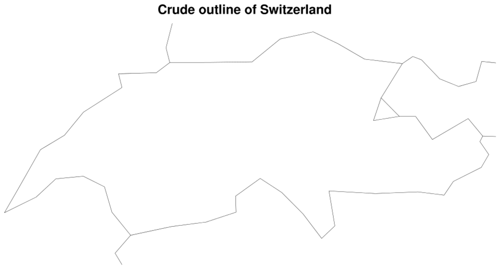
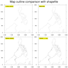
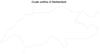
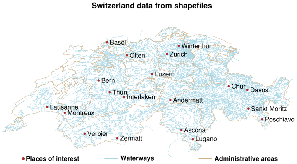 shapefiles_6.ncl:
This example uses a script very similar to example 3 above for South
America to draw the canton outlines for Switzerland. The first frame
shows the default map outline for Switzerland (admittedly not very good),
and the second frame shows the data from the shapefile.
shapefiles_6.ncl:
This example uses a script very similar to example 3 above for South
America to draw the canton outlines for Switzerland. The first frame
shows the default map outline for Switzerland (admittedly not very good),
and the second frame shows the data from the shapefile.
The point is to show that shapefiles tend to have similar formats, and hence you can take a script and easily modify it to draw the outlines you're interested in.
In this example, the outlines are drawn with polylines, and the places of interest with text strings and polymarkers.
With versions 6.1.2 or earlier of NCL, if you try to plot a lot of individual line segments or text strings using gsn_add_polyxxxx functions, then you may want to consider using gsn_polyline instead of gsn_add_polyline, gsn_polymarker instead of gsn_add_polymarker, and gsn_text instead of gsn_add_text.
With version 6.2.0 of NCL, drawing polylines and polygons is much faster. Markers and text may still be slow.
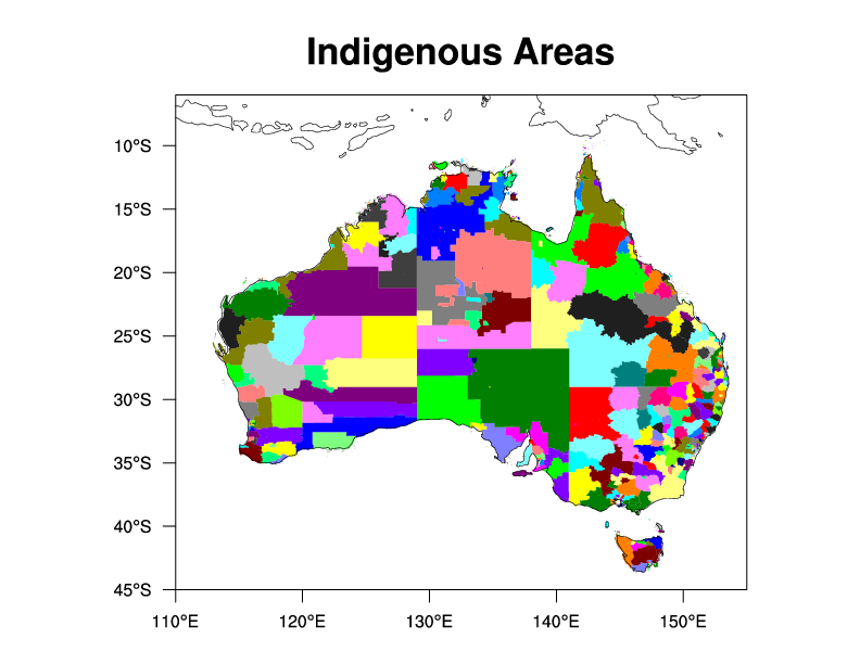
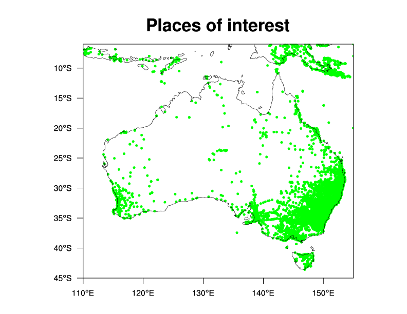
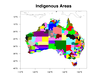
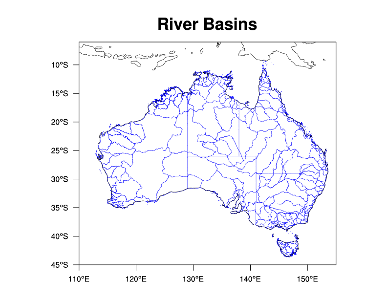 shapefiles_7.ncl:
This script uses several shapefiles to draw river basins, points of
interest, and indigenous areas in Australia. The shapefiles were
downloaded from several locations. See the comments in
the script for details.
shapefiles_7.ncl:
This script uses several shapefiles to draw river basins, points of
interest, and indigenous areas in Australia. The shapefiles were
downloaded from several locations. See the comments in
the script for details.
The routines gsn_add_shapefile_polygons, gsn_add_shapefile_polylines, and gsn_add_shapefile_polymarkers are used to attach the shapefile information.
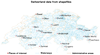
 shapefiles_8.ncl /
shapefiles_8_panel.ncl:
This script uses four shapefiles downloaded from
http://www.gadm.org/country
to draw various administrative areas for India.
shapefiles_8.ncl /
shapefiles_8_panel.ncl:
This script uses four shapefiles downloaded from
http://www.gadm.org/country
to draw various administrative areas for India.
 shapefiles_9.ncl:
This uses the shapefile Example 4.
This demonstrates calculating an areally weighted mean time series
for an irregularly shaped region. As in Example 4, an array containing
only the desired locations inside the shapefile is created. All other
grid points are set to _FillValue. Specifially, this computes the
areal mean time series of monthly precipitation for the Mississippi
River Basin. The data is the monthly GPCP.
shapefiles_9.ncl:
This uses the shapefile Example 4.
This demonstrates calculating an areally weighted mean time series
for an irregularly shaped region. As in Example 4, an array containing
only the desired locations inside the shapefile is created. All other
grid points are set to _FillValue. Specifially, this computes the
areal mean time series of monthly precipitation for the Mississippi
River Basin. The data is the monthly GPCP.
 mask_12.ncl: This example shows how
to use a shapefile that contains polygon outlines to create a data
mask for a variable with 1D coordinate arrays. The mask array is then
written to a copy of the input file. [This script
requires shapefile_utils.ncl.]
mask_12.ncl: This example shows how
to use a shapefile that contains polygon outlines to create a data
mask for a variable with 1D coordinate arrays. The mask array is then
written to a copy of the input file. [This script
requires shapefile_utils.ncl.]
In this case, the shapefile contains coastal outlines, which a land mask is created from. See the function "create_mask_from_shapefile" in the "mask_12.ncl" script. This function only works for data that contains coordinate arrays. You will need to modify it to work with curvilinear or unstructured data.
You should be able to use any shapefile that contains polygon data (point and polyline data won't work) to create the desired mask.
The shapefile used in this example was part of a compressed file,
"GSHHS_shp_2.2.0.zip", downloaded from:
http://www.ngdc.noaa.gov/mgg/shorelines/data/gshhs/oldversions/version2.2.0
You need to uncompress it with the "unzip" command. You can use any of the other shapefiles that are included with this file, but they are potentially a higher resolution, and hence creating the mask will take longer.
 shapefiles_10.ncl /
shapefiles_NM_10.ncl: These
examples show how to plot polygon data from a shapefile containing
geologic units and structural features in Colorado and New Mexico. The shapefiles were
downloaded from
http://mrdata.usgs.gov/geology/state/.
shapefiles_10.ncl /
shapefiles_NM_10.ncl: These
examples show how to plot polygon data from a shapefile containing
geologic units and structural features in Colorado and New Mexico. The shapefiles were
downloaded from
http://mrdata.usgs.gov/geology/state/.
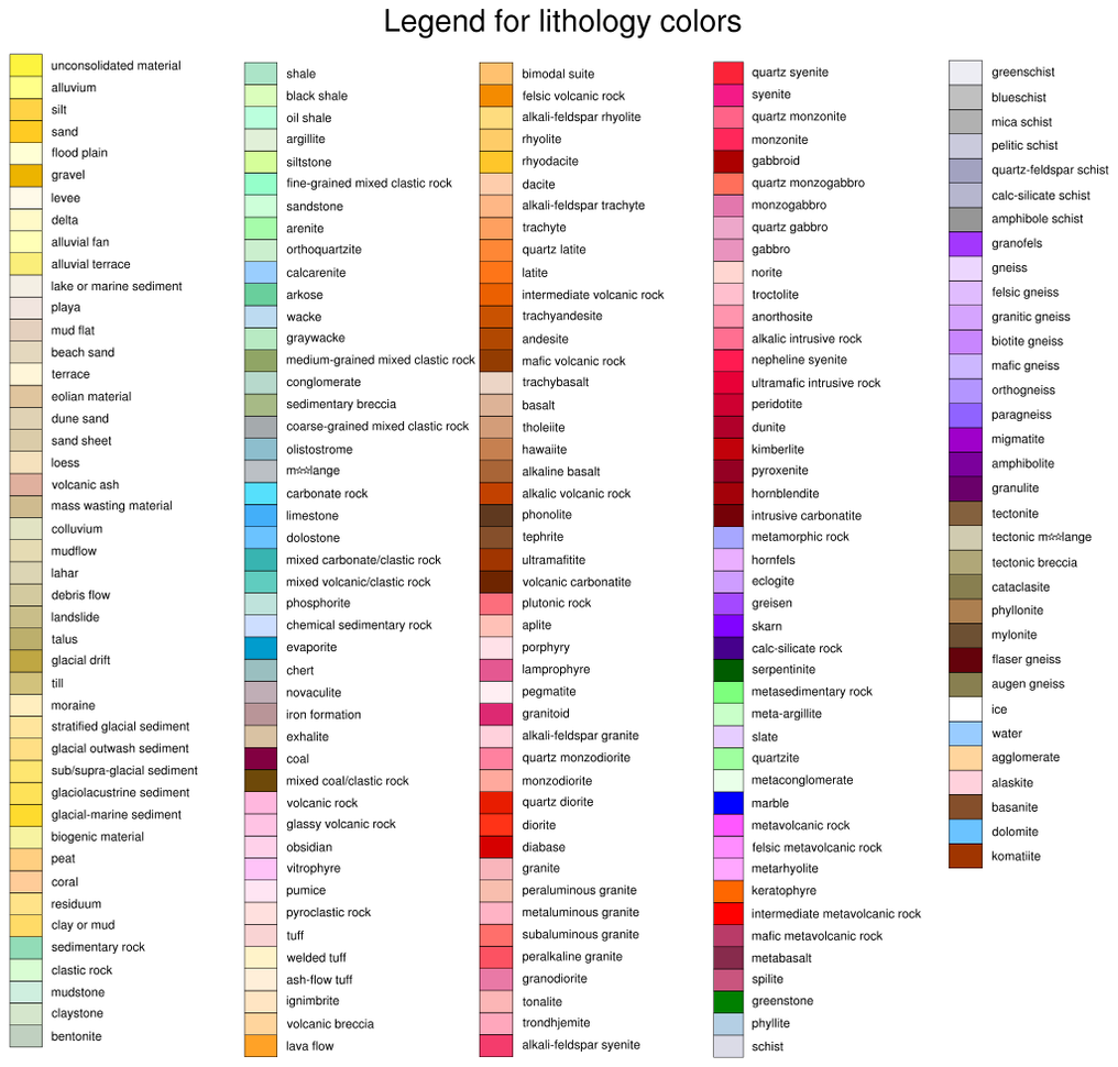
The shapefile data came with a suggested lithologic color map: http://mrdata.usgs.gov/catalog/lithclass-color.php, which shows which colors to use for which rock type. This example draws the lithologic color map on a separate frame, using several labelbars.
In order to use the suggested color map, the gsn_add_shapefile_polygons procedure was copied from the $NCARG_ROOT/lib/ncarg/nclscripts/csm directory, and then modified as needed.
The New Mexico image additionally adds fault lines.
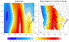
 shapefiles_11.ncl: This
example shows how to use a shapefile that contains an outline of the
United States to create a land mask. The land mask is written to a
NetCDF file so you can use it later for masking other variables on the
same grid.
shapefiles_11.ncl: This
example shows how to use a shapefile that contains an outline of the
United States to create a land mask. The land mask is written to a
NetCDF file so you can use it later for masking other variables on the
same grid.
This script calls shapefile_mask_data, which is in the shapefile_utils.ncl script. See the description of this function for important information.
Two USA shapefiles were tried with this example. The "gz_2010_us_020_00_5m.shp" shapefile is from http://www.census.gov/geo/www/cob/ and the "nationalp010g.shp" shapefile is from http://nationalmap.gov/small_scale/mld/1natlp.html. The census one is smaller and hence the script runs much faster on this one (200+ wall seconds versus 17 wall clock seconds). Which file you use depends on how fine your original grid is, and how good of a mask you need.
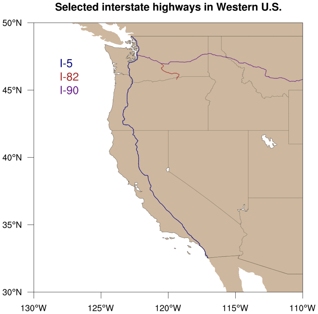
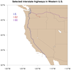
 shapefiles_12.ncl /
shapefiles_12b.ncl: This
example shows how to
modify gsn_add_shapefile_polylines
to have it draw only a subset of the features in the given shapefile.
shapefiles_12.ncl /
shapefiles_12b.ncl: This
example shows how to
modify gsn_add_shapefile_polylines
to have it draw only a subset of the features in the given shapefile.
See references to "feature_names", "vname", and "vlist" in the "gsn_add_shapefile_polylines_subset" function at the top of the NCL script.
The shapefile contains Interstate Highways, and only the primary interstate highways (I-5, I-82, and I-90) in Western United States are drawn. (Special thanks to Dave Allured for his improvement of this script to correctly plot all highway segments with complex entries, like "I- 5, US 30".)
The shapefile was downloaded from http://www.nws.noaa.gov/geodata/catalog/transportation/html/interst.htm.
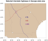
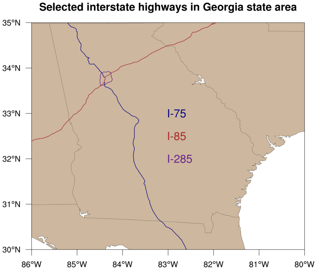
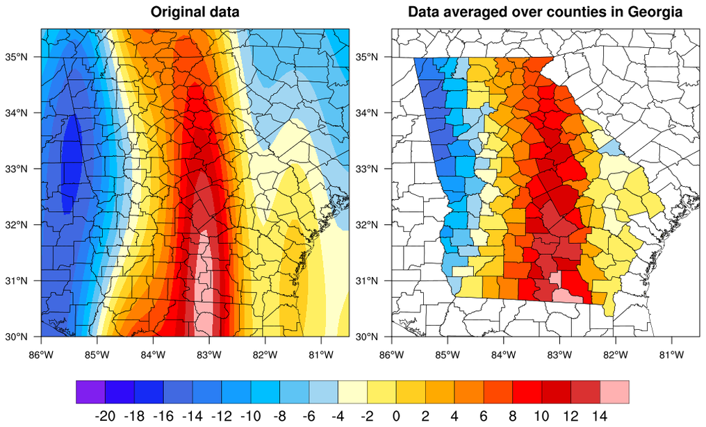 shapefiles_13.ncl: This
example shows how to use shapefile data to collect lat/lon data points
in each county of Georgia, and take an average of all the data values
in that county. Based on each county average, a fill color is assigned
and the county is filled using
modify gsn_add_polygon.
shapefiles_13.ncl: This
example shows how to use shapefile data to collect lat/lon data points
in each county of Georgia, and take an average of all the data values
in that county. Based on each county average, a fill color is assigned
and the county is filled using
modify gsn_add_polygon.
The gc_inout function is used to collect lat/lon pairs that fall in each county. Since this function can be slow if you are checking a lot of points, a number of "if" statements are included to prevent unnecessary calls to this function.
The county outlines for Georgia come from the USA_adm2.shp shapefile, which was downloaded from http://www.gadm.org/country.
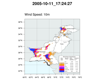
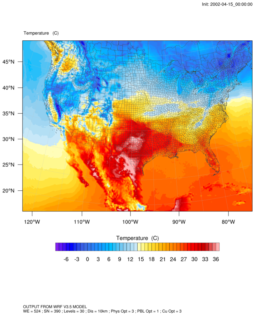 shapefiles_14.ncl: This
example shows how to add shapefile outlines to an existing WRF
contour/map plot.
shapefiles_14.ncl: This
example shows how to add shapefile outlines to an existing WRF
contour/map plot.
In order to attach the shapefile outlines to the plot, you need to set "pltres@PanelPlot = True" so that wrf_map_overlays doesn't remove the contour plot. You can then use gsn_add_shapefile_polylines to add the shapefile outlines.
The country outline for USA was downloaded from http://www.gadm.org/country.
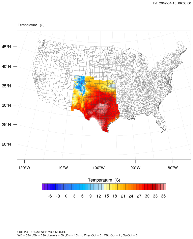
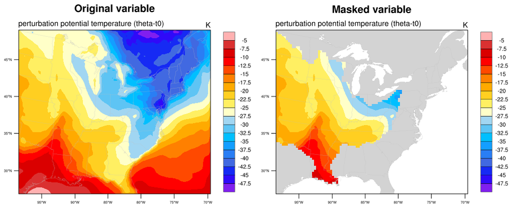
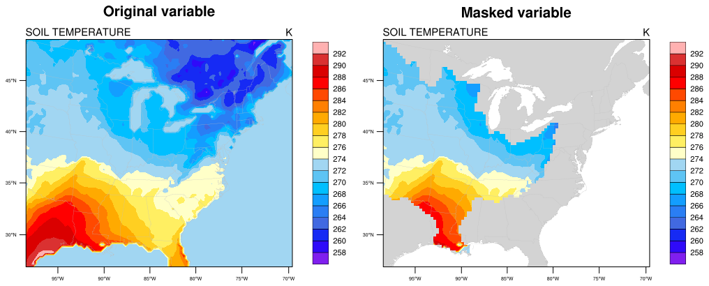
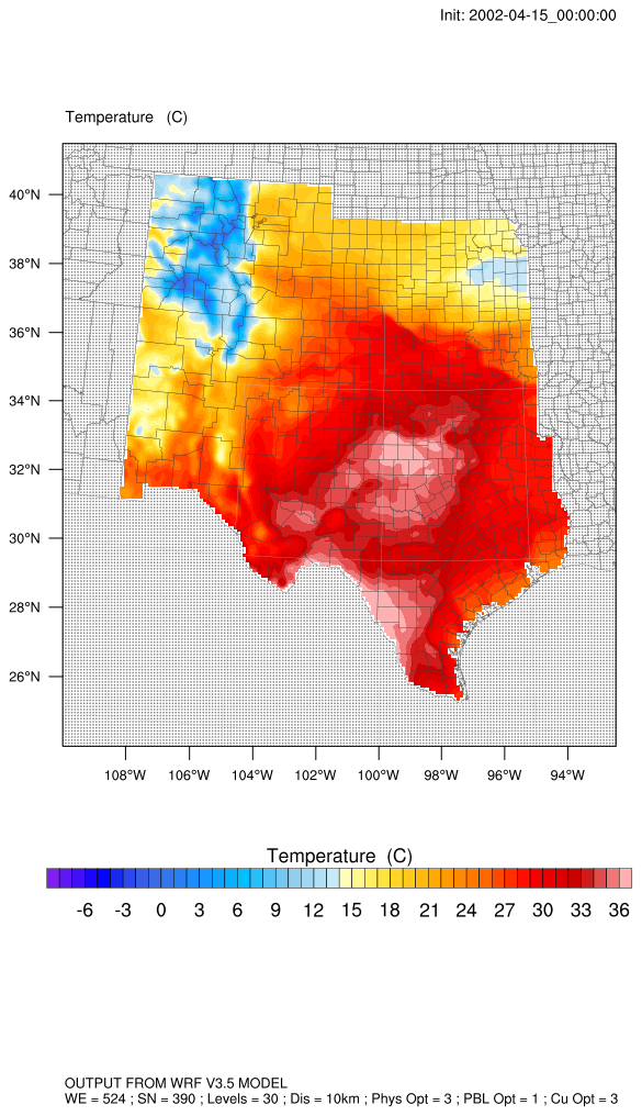 shapefiles_14_mask.ncl: This
example is similar to the previous one, except it masks the WRF "hgt"
variable against a select list of U.S. states outlines from the
shapefile.
shapefiles_14_mask.ncl: This
example is similar to the previous one, except it masks the WRF "hgt"
variable against a select list of U.S. states outlines from the
shapefile.
This script calls shapefile_mask_data, which is in the shapefile_utils.ncl script. See the description of this function for important information.
The outlines for the U.S. states comes from the USA_adm2.shp shapefile, which was downloaded from http://www.gadm.org/country.
The first frame is the unzoomed variable, and the second frame shows how to zoom in on the area of interest using the special "ZoomIn" WRF resource.
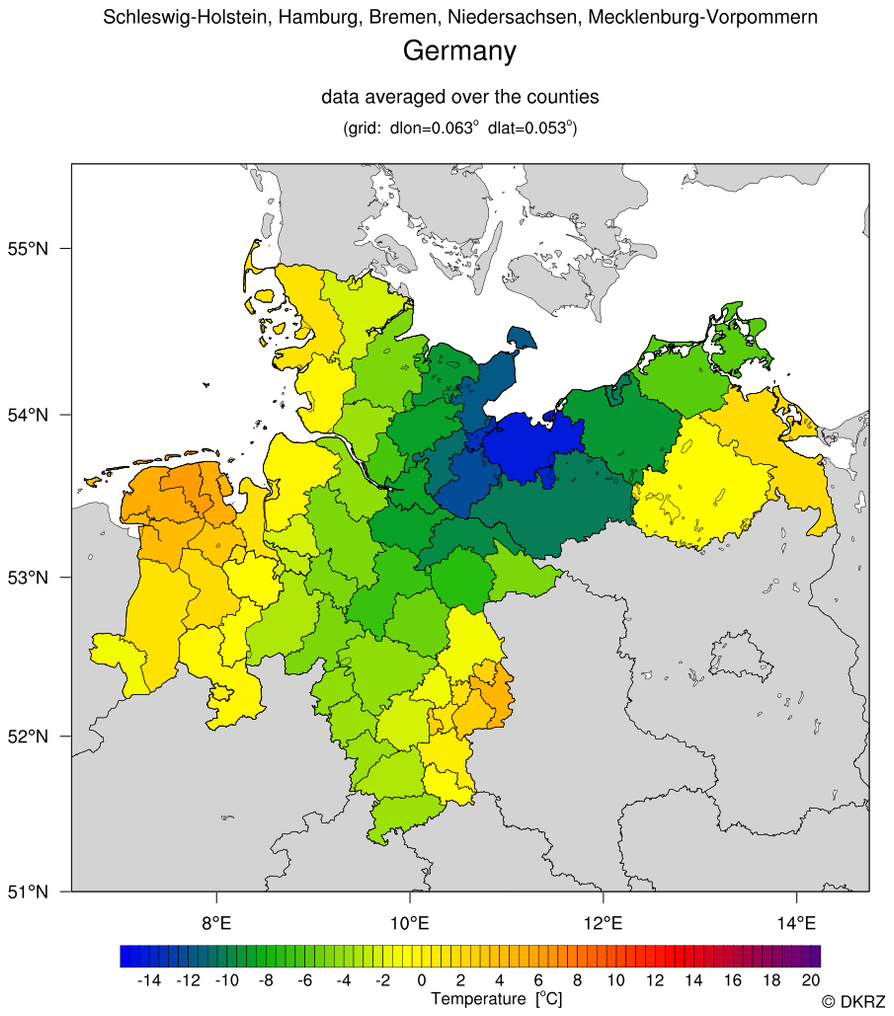 Germany_coastal_counties_DEU_adm.ncl:
This script, contributed by Karin Meier-Fleischer
of Deutsche Klimarechenzentrum
(DKRZ), shows how to use the DEU_adm3.shp shapefile downloaded
from http://www.gadm.org/country
to average data over coastal counties of Germany.
Germany_coastal_counties_DEU_adm.ncl:
This script, contributed by Karin Meier-Fleischer
of Deutsche Klimarechenzentrum
(DKRZ), shows how to use the DEU_adm3.shp shapefile downloaded
from http://www.gadm.org/country
to average data over coastal counties of Germany.
You can customize what outlines are drawn by using command line options. Examples:
- Coastal region
ncl 'subregion="6.5,14.75,50.,55.5"' Germany_coastal_counties_DEU_adm.ncl - Draw "Schleswig-Holstein" (default) and plot only the sub-region
ncl 'subregion="7.8,11.9,53.0,55.3"' Germany_coastal_counties_DEU_adm.ncl - Draw "Schleswig-Holstein" (default) but don't draw the border of all states
ncl 'states_border=False' Germany_coastal_counties_DEU_adm.ncl - Select the state "Hessen" but don't draw the borderline of Germany
ncl 'state_name="Hessen"' 'country_border=False' Germany_coastal_counties_DEU_adm.ncl
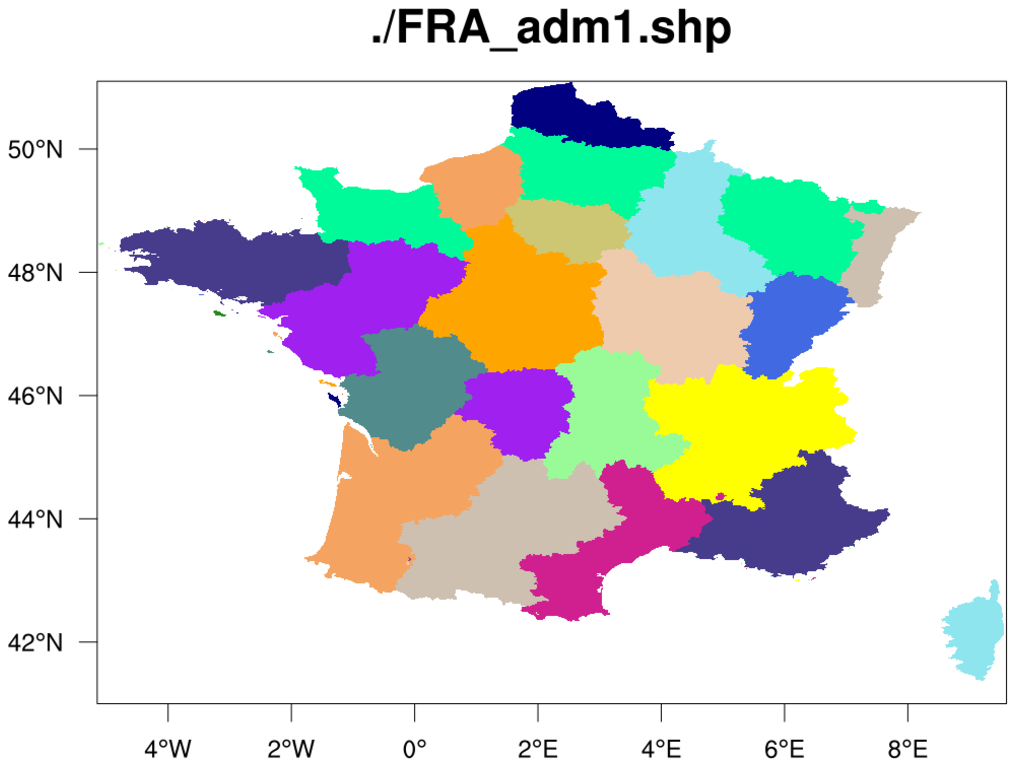 France_1.ncl /
France_2.ncl /
France_3.ncl:
The purpose of this example is to demonstrate the use of the
gsSegments and
gsColors
resources added in
added in version 6.2.0,
and how much routines like
gsn_add_shapefile_polygons,
gsn_add_shapefile_polylines,
gsn_add_polyline,
gsn_add_polygon
have been sped-up
in version 6.2.0.
France_1.ncl /
France_2.ncl /
France_3.ncl:
The purpose of this example is to demonstrate the use of the
gsSegments and
gsColors
resources added in
added in version 6.2.0,
and how much routines like
gsn_add_shapefile_polygons,
gsn_add_shapefile_polylines,
gsn_add_polyline,
gsn_add_polygon
have been sped-up
in version 6.2.0.
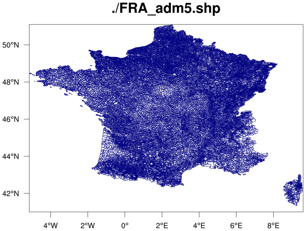
If you run the France_1.ncl script with the France administrative shapefiles downloaded from gadm.org/country, you will see significant speed-up mostly for the "FRA_adm5.shp" file, which has 36,612 features to draw:
--------------------------
NCL V6.1.2 timing results:
--------------------------
. . . SNIP . . .
---> Drawing FRA_adm/FRA_adm5.shp...
     207.032 CPU seconds

--------------------------
NCL V6.2.0 timing results:
--------------------------
. . . SNIP . . .
---> Drawing FRA_adm/FRA_adm5.shp...
     2.87449 CPU seconds
Note: this scrip actually generates six images. The timing results and the image displayed above are from running this script with the "do" loop changed to "do i=5,5".
The France_2.ncl script produces identical plots, only it uses gsn_add_polyline instead of gsn_add_shapefile_polylines. This script will only work with NCL V6.2.0, because it references the gsSegments resource directly.
The France_3.ncl script draws the "FRA_adm1.shp" shapefile as filled polygons, using gsColors to specify a fill color for each segment.
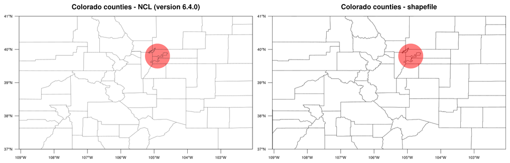
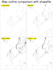
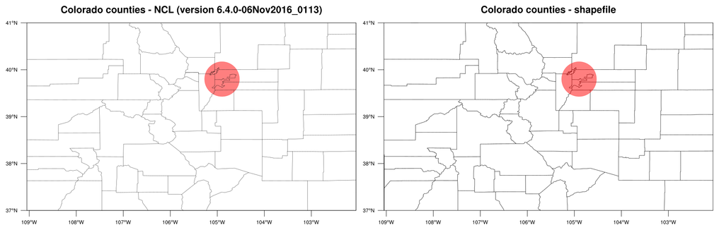 shapefiles_15.ncl: This
example is another one showing the difference between map outlines in
NCL and map outlines added from a shapefile. The first plot in the
panel shows the counties of Colorado as plotted from NCL, and the
second plot shows the counties as plotted from the USA_adm2 shapefile
downloaded from
http://www.gadm.org/country.
shapefiles_15.ncl: This
example is another one showing the difference between map outlines in
NCL and map outlines added from a shapefile. The first plot in the
panel shows the counties of Colorado as plotted from NCL, and the
second plot shows the counties as plotted from the USA_adm2 shapefile
downloaded from
http://www.gadm.org/country.
The left image is from running NCL V6.3.0 on this script. The right image is from running NCL V6.4.0.
In NCL versions 6.3.0 and earlier, the NCL outlines will not show the county of Broomfield or the updated counties around Denver. In NCL version 6.4.0, the NCL map databases were updated to reflect the current Colorado counties.
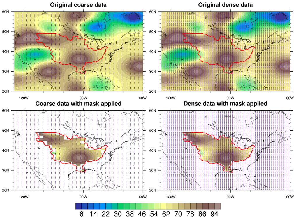 shapefiles_16.ncl: This
example shows the effect that shapefile masking will have on both a
coarse (32 x 64) and fine (64 x 128) grid.
shapefiles_16.ncl: This
example shows the effect that shapefile masking will have on both a
coarse (32 x 64) and fine (64 x 128) grid.
The gsn_coordinates procedure is used to draw the lat/lon grid as a set of markers.
See example 21 below for an example that compares masking data using shapefile_mask_data, and masking data by drawing the undesired areas in white.
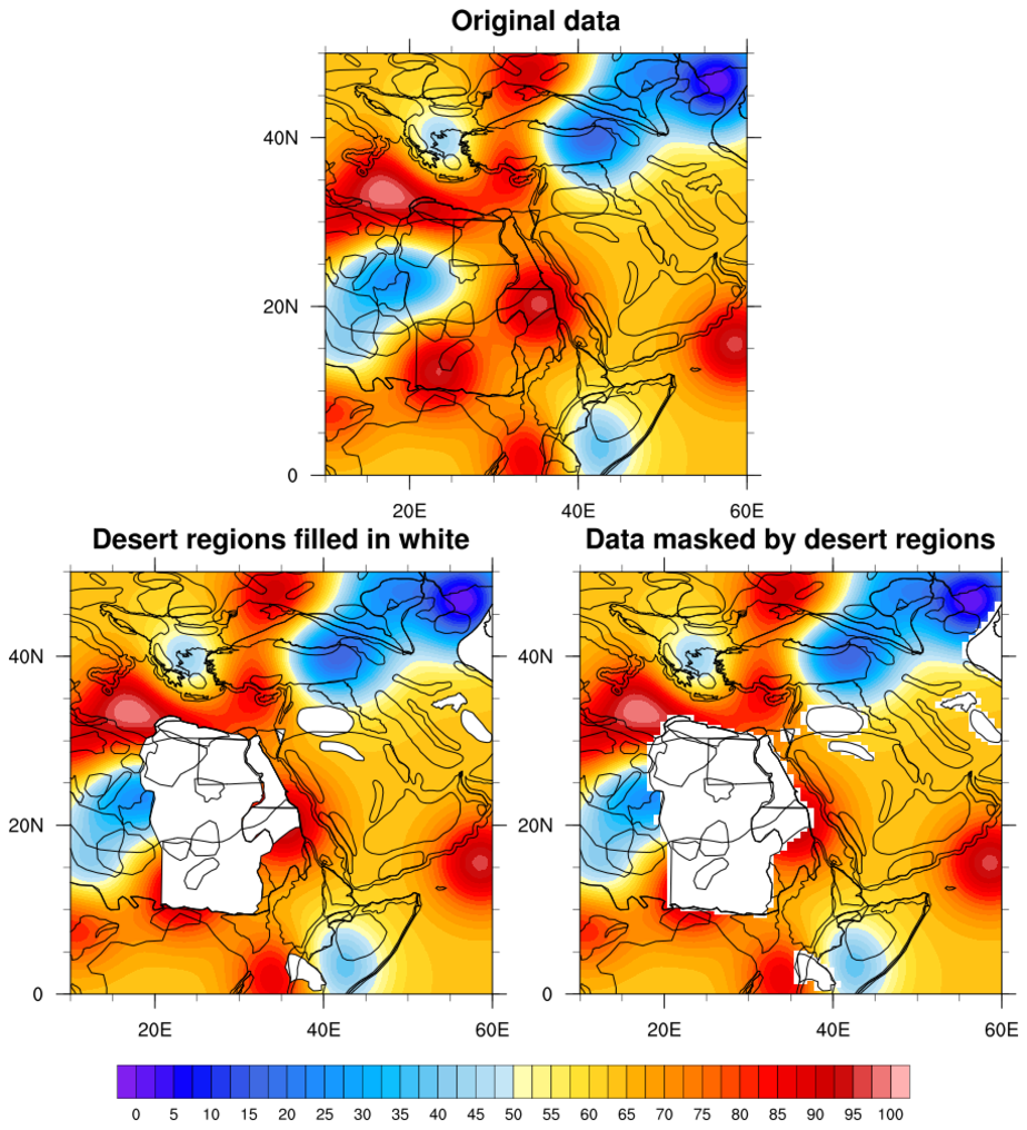 shapefiles_17.ncl: This
example shows two ways to mask data based out outlines in a
shapefile: one is to use the shapefile_mask_data function
mentioned in previous examples, and another is to simply fill
in the undesired outlines in white over the original
contour data, effectively masking it.
shapefiles_17.ncl: This
example shows two ways to mask data based out outlines in a
shapefile: one is to use the shapefile_mask_data function
mentioned in previous examples, and another is to simply fill
in the undesired outlines in white over the original
contour data, effectively masking it.
The shapefile_mask_data function is in the shapefile_utils.ncl script. See the description of this function for important information.
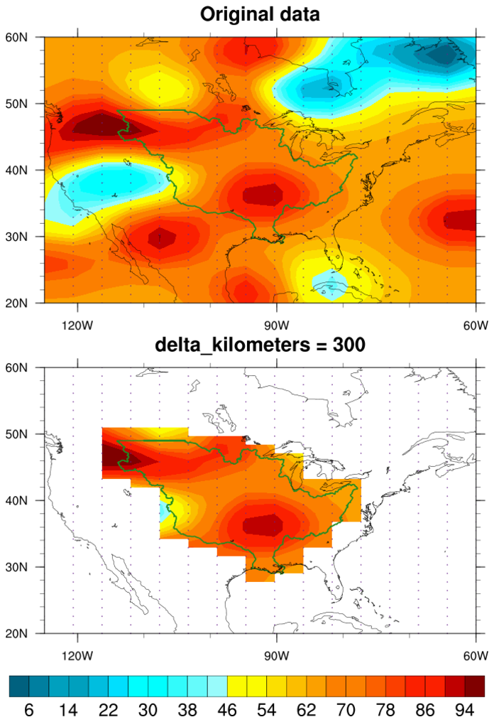 shapefiles_18.ncl: This
example uses a modified version of "shapefile_mask_data" to
mask data based on a shapefile outline, and a "delta" distance
(in km) outside the shapefile outline. See "delta_kilometer"
in the script.
shapefiles_18.ncl: This
example uses a modified version of "shapefile_mask_data" to
mask data based on a shapefile outline, and a "delta" distance
(in km) outside the shapefile outline. See "delta_kilometer"
in the script.
This is useful if you want to keep some of your original data points that fall just outside a shapefile outline.
This script requires shapefile_mask_data_mod.ncl.
 shapefiles_19.ncl:
This example shows how to either mask (retain) or remove data, based on a shapefile
outline. We get a lot of questions on this topic, so we decided to create a very
basic example that shows both types of masking.
shapefiles_19.ncl:
This example shows how to either mask (retain) or remove data, based on a shapefile
outline. We get a lot of questions on this topic, so we decided to create a very
basic example that shows both types of masking.
This example uses the shapefile_mask_data function found shapefile_utils.ncl. See the description of this function for important information.
In order to mask data against outlines in a shapefile, you must provide the name of a variable on the shapefile that contains the list of names or values you want to mask against.
For example, here, the "USA_adm1.shp" shapefile is being used, which has a "NAME_1" string array containing feature names that are simply the U.S state names: "Alabama", "New Mexico", etc. You can reference one or more of these strings to indicate you want to mask or keep data in these areas.
The shapefile_mask_data function, in the shapefile_utils.ncl script, allows you to set the special "keep" option to False, which will cause data to be removed rather than retained.
 shapefiles_20.ncl:
This example shows how to use the shapefile_mask_data function in
shapefile_utils.ncl
to return a mask array, and then apply this mask array to a variable
with multiple time steps. The special option "return_mask" is
set to True, telling the function to return the 0/1 mask array,
instead of returning the masked data itself.
shapefiles_20.ncl:
This example shows how to use the shapefile_mask_data function in
shapefile_utils.ncl
to return a mask array, and then apply this mask array to a variable
with multiple time steps. The special option "return_mask" is
set to True, telling the function to return the 0/1 mask array,
instead of returning the masked data itself.
The conform_dims function is used to conform the mask array to a 3D array, and then mask is used to apply the mask.
You can only do this kind of masking if your lat/lon grid remains the stationary across all time steps.
See the description of shapefile_mask_data for important information.
 shapefiles_21.ncl:
This example demonstrates two ways to mask data based on shapefile
outlines of interest.
shapefiles_21.ncl:
This example demonstrates two ways to mask data based on shapefile
outlines of interest.
The first plot shows the original data with no masking. The purple lines represent the shapefile areas that we want to apply the masking to.
The second plot shows the result of using the shapefile_mask_data function (in shapefile_utils.ncl) to mask the data based on an array of given areas to mask. (You can use strings or numeric types for the areas you want to mask, but the array values should match whatever type the variable is on the shapefile.) You will see the blockiness near the shapefile outlines, due to the fact that NCL will not contour data that is bordered by missing values. The black dots represent the WRF data that was kept by this function, and the red dots represent the data that was set to missing.
The third plot shows how to mask the data by filling the undesired areas in white. This is a bit of a pain, because you have to make sure you fill in all the undesired areas, and set various "draw order" resources to make sure things are drawn in the correct order. This method is only useful when doing graphics, and not if you need to mask the data for calculation purposes later.
Note that the third plot shows some white areas inside the purple shapefile outlines. This is due to the fact that the script set mpOceanFillColor to "white", which causes some shapefile areas to be covered up by the white ocean areas.

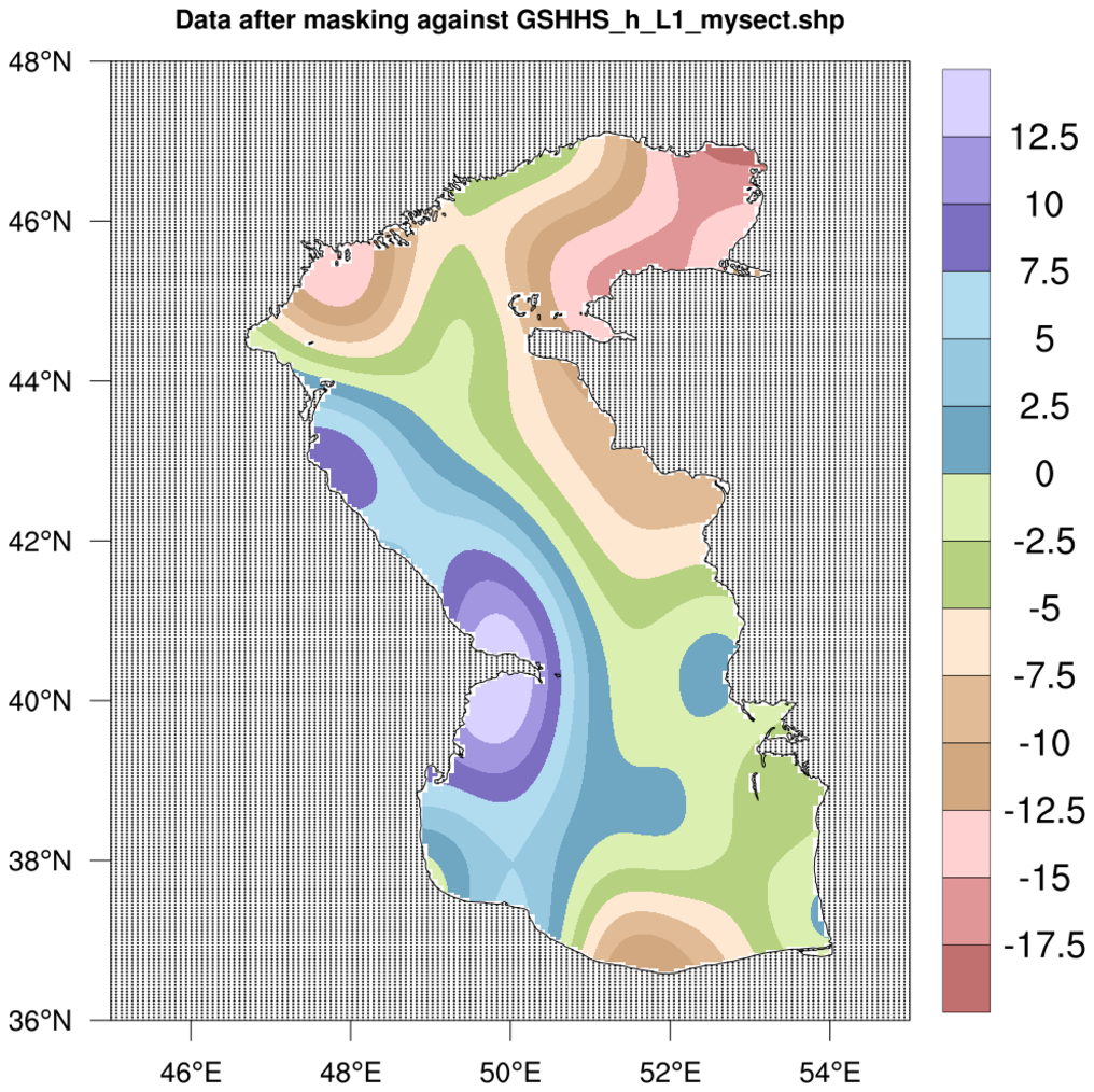
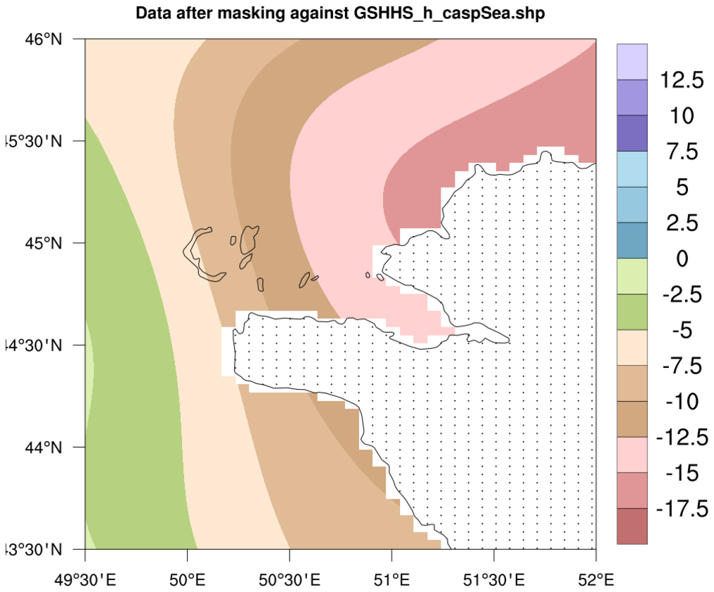
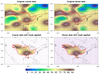
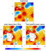
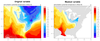
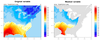
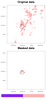
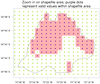
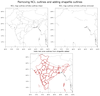
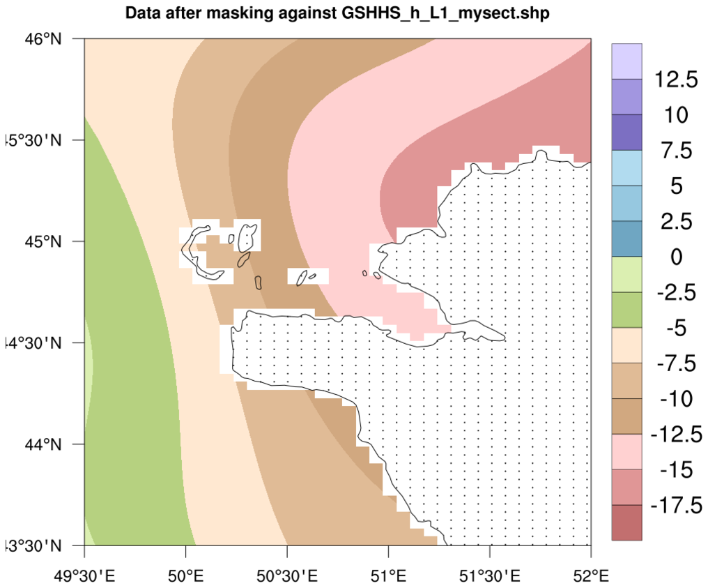 shapefiles_22.ncl: This
example shows how to use two different shapefiles to mask data. One
shapefile contains a single outline of the Caspian Sea, and the other
contains outlines of isles inside the Caspian Sea.
shapefiles_22.ncl: This
example shows how to use two different shapefiles to mask data. One
shapefile contains a single outline of the Caspian Sea, and the other
contains outlines of isles inside the Caspian Sea.
If you want to keep the data inside the Caspian Sea, but not inside the isles, then you need to mask the data twice: first by setting the "keep" attribute to True to keep the values inside the single outline, and second by setting "keep" to False to throw away values in the isle areas:
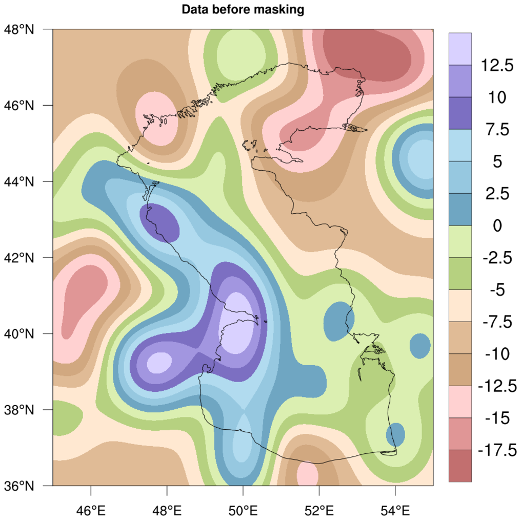
  opt      = True
  opt@keep = True   ; Keep values inside this shape
  data_mask_casp = shapefile_mask_data(data,caspian_shape_name,opt)

  opt@keep = False
  data_mask_isles = shapefile_mask_data(data_mask_casp,isles_shape_name,opt)
Image #1: The original data before masking
Image #2: The data after masking against the Caspian Sea outline. Note that the little isles still have data in them.
Image #3: The data after masking the previously-masked data against the isle outlines. Note that the isles no longer have data in them.
Images #4-5: Zoomed in versions of images #2-3.
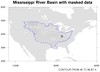
 shapefiles_23.ncl: This script
shows how to use shapefile_mask_data to create a mask array for
masking a WRF output variable against an outline in a shapefile. It
then uses this mask array to mask select variables on the file.
shapefiles_23.ncl: This script
shows how to use shapefile_mask_data to create a mask array for
masking a WRF output variable against an outline in a shapefile. It
then uses this mask array to mask select variables on the file.
Creating a mask array from a shapefile can take a long time if you have a big shapefile or lots of points to check. Once you have the mask array, use it with the mask function to mask other variables of the same size. This goes MUCH faster than using shapefile_mask_data. You can also write this mask array to a NetCDF file for use by other scripts.
Optionally, this script writes the masked variables to a new NetCDF file, and/or plots the original data versus the masked data for comparison.
This script uses a Mississippi River Basin shapefile (mrb.xxx) for demonstrative purposes. You should use your own shapefile data, but you can download the mrb files if needed.
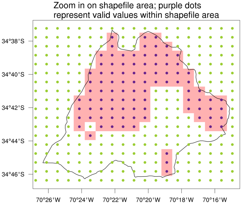
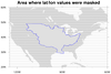
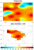
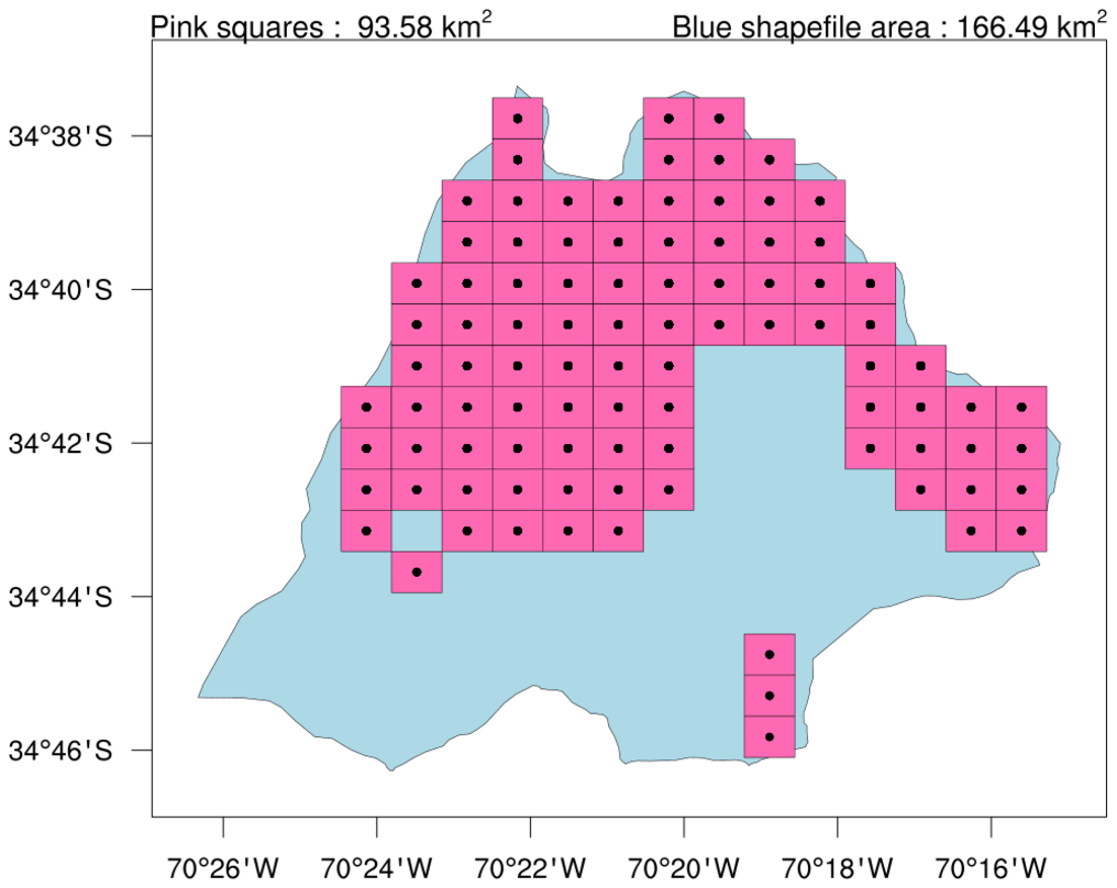 shapefiles_24.ncl: This script
uses a shapefile outline to mask some data, and then calculates the
approximate area (in km^2) of the valid data that was retained
inside the shapefile area.
shapefiles_24.ncl: This script
uses a shapefile outline to mask some data, and then calculates the
approximate area (in km^2) of the valid data that was retained
inside the shapefile area.
It does this by generating a series of quadrilaterals around every lat/lon point of valid data, and calling gc_qarea to get a sum of the area of all of them. This is only a rough approximation of the actual area of the data, which you can see by the pink squares in the third image.
For comparison purposes, the area (in km^2) of shapefile outline was also calculated, using area_poly_sphere.
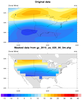
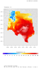
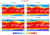
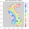
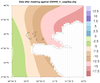
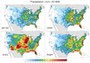
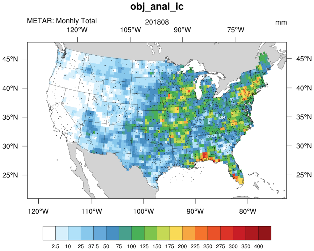 shapefiles_25.ncl:
Read hourly METAR precipitation values for August 2018 at station locations.
Calculate monthly total precipitation at each station. Use Barnes iterative
correction (obj_anl_ic) to regrid the
data onto a user defined grid. Use a shape file to create grid mask to eliminate
values outside the coterminus USA. Plot as 'raster' to illustrate the underlying
grid resolution.
shapefiles_25.ncl:
Read hourly METAR precipitation values for August 2018 at station locations.
Calculate monthly total precipitation at each station. Use Barnes iterative
correction (obj_anl_ic) to regrid the
data onto a user defined grid. Use a shape file to create grid mask to eliminate
values outside the coterminus USA. Plot as 'raster' to illustrate the underlying
grid resolution.
The United States Census cartographic boundary shapefile, cb_2018_us_nation_5m.zip, was downloaded from: https://www.census.gov/geographies/mapping-files/2018/geo/carto-boundary-file.html
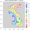
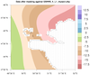
 shapefiles_26.ncl:
Similar to shapefiles_25 except values from four different sources
(METAR, HRR, GOES, Stage4) are used. The mask file created and saved
in shapefiles_25 is used to mask values outside the coterminus USA.
Plot as a panel.
shapefiles_26.ncl:
Similar to shapefiles_25 except values from four different sources
(METAR, HRR, GOES, Stage4) are used. The mask file created and saved
in shapefiles_25 is used to mask values outside the coterminus USA.
Plot as a panel.
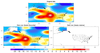
 maponly_30.ncl: This script
shows how to use the mpMaskOutlineSpecifiers
to remove the outlines of India, while keeping outlines from surrounding
countries. In the third plot, meteorological subdivisions of India
were added using a shapefile downloaded off the web.
maponly_30.ncl: This script
shows how to use the mpMaskOutlineSpecifiers
to remove the outlines of India, while keeping outlines from surrounding
countries. In the third plot, meteorological subdivisions of India
were added using a shapefile downloaded off the web.