NCL Home>
Application examples>
Data Analysis ||
Data files for some examples
Example pages containing:
tips |
resources |
functions/procedures
NCL: Madden Julian Oscillation Climate Variability
Prior to NCL 6.2.0, the following four libraries needed to be loaded prior to invoking the diagnostic scripts:
   load "$NCARG_ROOT/lib/ncarg/nclscripts/csm/gsn_code.ncl"
   load "$NCARG_ROOT/lib/ncarg/nclscripts/csm/gsn_csm.ncl"
   load "$NCARG_ROOT/lib/ncarg/nclscripts/csm/contributed.ncl"
   load "$NCARG_ROOT/lib/ncarg/nclscripts/csm/diagnostics_cam.ncl"
From NCL 6.2.0 onward, only the following need be loaded:
load "$NCARG_ROOT/lib/ncarg/nclscripts/csm/diagnostics_cam.ncl"
The scripts below are intended to be 'guides' to usage. They may
work directly but, generally, the user will have to make
some changes to the scripts. For example, the changes may involve
making the time variable similar to those used in the examples.
The
US-CLIVAR MJO working
group developed diagnostics for objectively evaluating the MJO.
Unfortunately, the original
official US-CLIVAR MJO diagnostics website is no longer
available. It provided data, C-shell and GrADS scripts and Fortran code to
implement and display the suggested diagnostics. The NCL examples presented below
perform the suggested diagnostics.
Reference
   MJO Simulation Diagnostics
   Waliser et al.
   2009, J. Clim.,  22: 3006-3030
   DOI: 10.1175/2008JCLI2731.1

   MJO simulation in CMIP5 climate models: MJO skill metrics and process-oriented diagnosis
   Ahn M-S et al.
   2017, Climate Dynamics, 49: 4023-4045
MJO Diagnostic Semantics
The diagnostics are categorized into two (really, three) levels:
- Level 1: Diagnostics meant to provide a basic indication
of the spatial and temporal intraseasonal variability that can be
easily understood and/or calculated by the non-MJO expert.
- Level 2: Diagnostics that provide a more comprehensive
diagnosis of the MJO through multivariate EOF analysis and
frequency wave-number decomposition.
- Other or Supplemental:
Diagnostics that provide additional measures that have in some
cases been found to play an important role in MJO simulation
fidelity (e.g., mean state) or characterize the manner the MJO
interacts with other important weather/climate processes (e.g., ENSO)
Observational Datasets used here [mainly netCDF]
       daily and monthly mean NCEP winds
       daily and monthly NOAA  Interpolated OLR
       monthly and pentad CMAP
       monthly GPCP
       daily GPCP
       pentad GPCP
       daily TRMM
       monthly OI SST V2
Anomalies and Prewhitening
Generally, it is suggested that the diagnostics
should be performed on daily anomalies.
Unfiltered anomalies are computed by subtracting the climatological
daily (or pentad where appropriate) means calculated using all years
of the data.
There are two approaches: (a) Compute the climatology
and the anomalies 'on-the-fly', or, (b) Compute
anomalies and save them to a file. For convenience, the latter
approach is used in many of the examples.
Removing the climatological annual cycle is a form a "prewhitening".
Prewhitening is the the removal of known signals prior to
analysis so they will not confound the interpretation of the results.
For example, a model may have a known bias. This should be removed
prior to applying the methods shown below.
Active MJO periods and MJO Forecasts
When focusing on a specific period, several examples use the winter of
1996-1997. This was a particulary active period and is sometimes
considered the "gold standard" for MJO activity.
Matt Wheeler (CAWCR: The Centre for Australian Weather and Climate Research)
has several WWW links that perform real-time monitoring of the MJO.
These show other periods of strong MJO activity. NOAA provides access to
experimental MJO forecasts.
Carl Schreck ( CICS:
Cooperative Institute for Climate and Satellites) has additional WWW site for
Monitoring the MJO and Tropical Waves.
Lanczos Filter Weights
 When needed, the weights for the suggested 20-100 day bandpass Lanczos filter
are generated 'on-the-fly' using:
When needed, the weights for the suggested 20-100 day bandpass Lanczos filter
are generated 'on-the-fly' using:
  ihp      = 2                             ; bpf=>band pass filter
  nWgt     = 201
  sigma    = 1.0                           ; Lanczos sigma
  fca      = 1./100.
  fcb      = 1./20.
  wgt      = filwgts_lanczos (nWgt, ihp, fca, fcb, sigma )
The band pass filter (BPF) weights are applied via a weighted running average.
For example, an array x(time,lat,lon) would be filtered via
xBPF = wgt_runave_Wrap (x(lat|:, lon|:, time|:), wgt, 0)
The resulting array would be xBPF(lat,lon,time).
More
filter examples
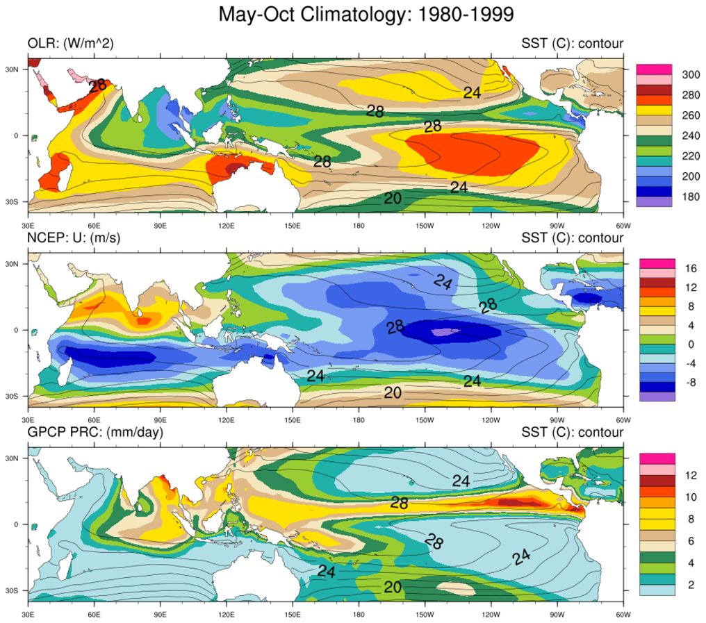
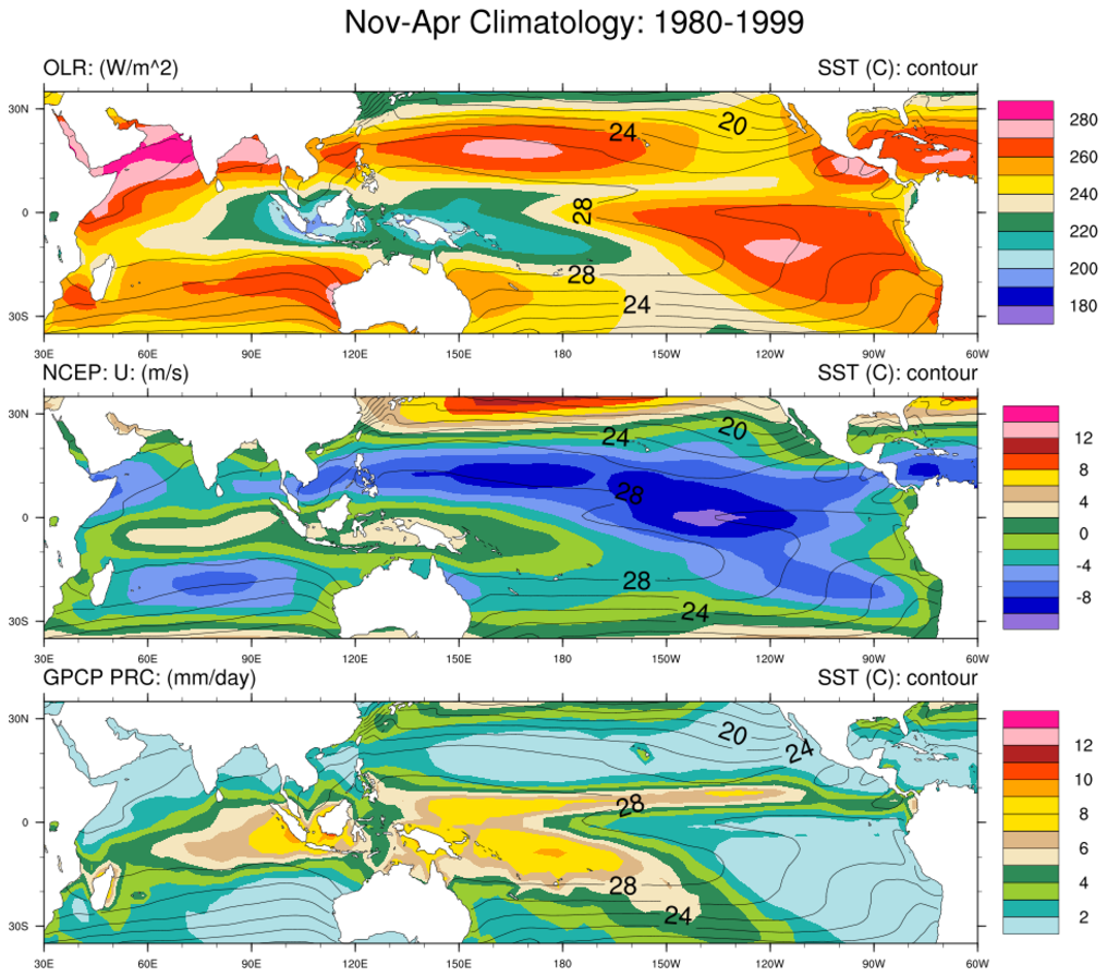
 mjoclivar_1.ncl
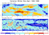
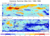
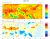
:
This example illustrates plotting what is referred to as the
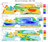
Mean State which is a supplemental diagnostic. Specifically:
     (a) Read files containing year-month data,
     (b) Create climatologies spanning user specified years
     (c) Plot November-April and May-October climatologies
                over a user specified region
 mjoclivar_2.ncl
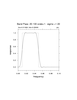
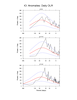
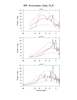
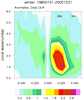
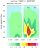
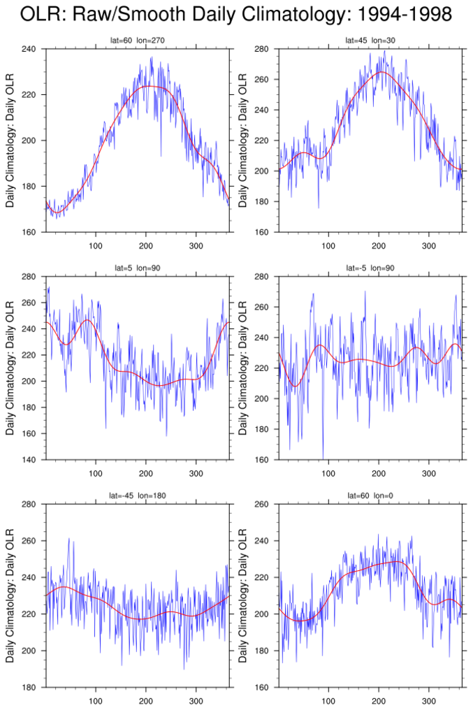
:
The MJO reference suggests using daily anomalies for the diagnostics.
The following illustrates the process of creating anomalies.
Calculate the daily mean annual cycle and daily anomalies from the mean
annual cycle. For illustration:
     (a) Read the raw daily data.
     (b) Compute raw and smoothed annual cycles
     (c) Create netCDF file containing the anomalies
     (d) Plots: (i) daily climatologies at different locations
               (ii) sample anomalies using smooth and raw climatologies
This example uses 26-years (1980-2005) of daily data.
The variability of the raw climatological day-to-day values is a direct
function of the number of years used to create the climatologies.
Generally speaking, using more/fewer years will result in
smaller/greater day-to-day variability. Note: the the
scales are different for each plot on the leftmost figure.
Which is the proper climatological daily annual
cycle to use: raw or smoothed?
It depends on your usage. The smoothed annual cycle
can be thought of as the values that would be obtained
if there was an infinite ensemble of data under the same
forcing conditions.
 mjoclivar_3.ncl
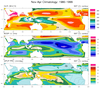
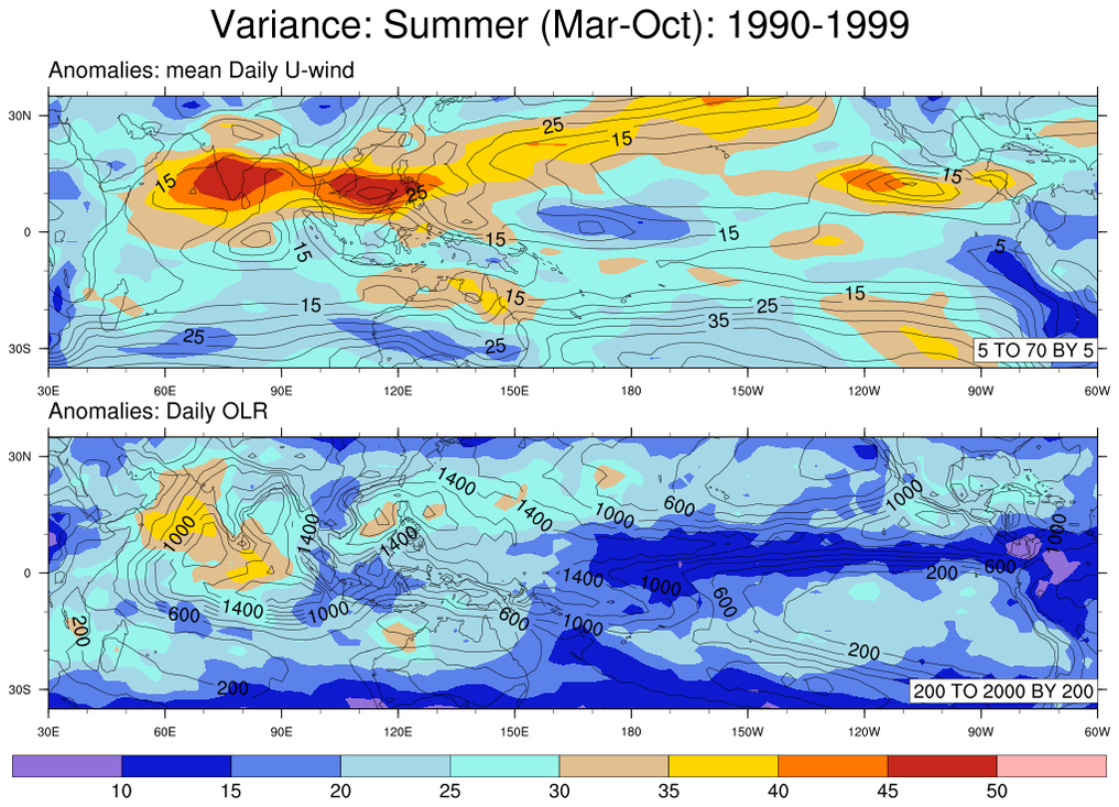
:
This example uses 10-years (1990-1999) of daily anomaly data
to compute seasonal variances and the ratio of the bandpass
variance to the unfiltered variance. Here, the base (color)
plot contains the *ratios*. The overlay plot (contour lines)
are the filtered variance ate each grid point.
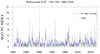
 mjoclivar_4.ncl
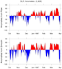
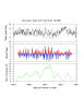
:
Use
band_pass_area_time to:
     (a) Create a single time series of areal averaged data
     (b) Band pass filter the resulting area averaged time series
     (c) Calculate a running 91-day variance of (b)
     (d) plot using band_pass_area_time_plot
Note: The MJO-WG recommended band pass filter is used. However, the
band_pass_area_time function can create and use other band pass weights.
 mjoclivar_6.ncl
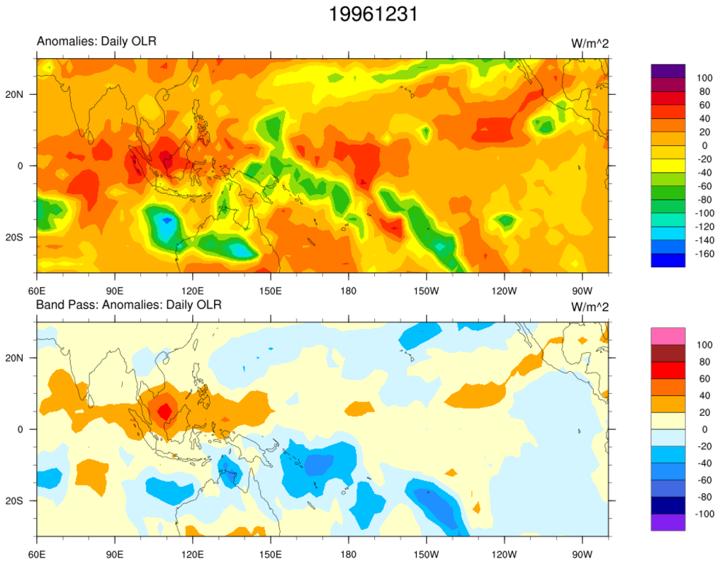
:
Create band-pass filtered time series at each lat/lon grid point via
band_pass_latlon_time. Plot the total anomaly pattern and the corresponding
band pass filtered pattern at a specific date.
Note: A movie could
readily be created.
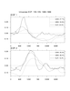
 mjoclivar_7.ncl
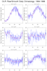
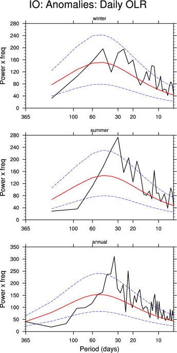
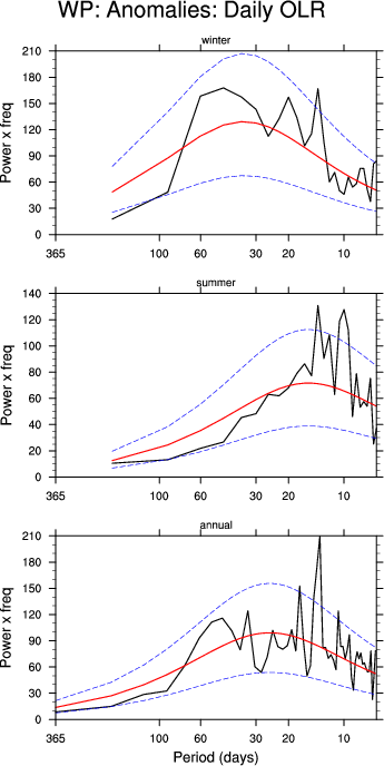
:
Unfiltered anomaly data are averaged over user specified
domains described in
Table 1
of the 'MJO Clivar' website.
The spectra are calculated separately for each season and
averaged across all years for the given season. The number of degrees
of freedom is approximately 2*(number of seasons). The null, 5% and 95%
red noise significance levels are included. Plot spectra with x-axis
as frequency with log scaling and y-axis as power times frequency.
The data are cosine area-weighted in latitude as specified
by MJO Clivar.
The mjo_spectra procedure is a driver which computes
and plots the seasonally averaged spectra.
The seasonal spectra are calculated via the mjo_spectra_season function.
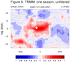
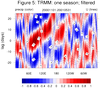
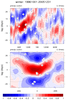
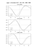
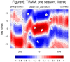 mjoclivar_8.ncl
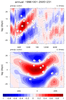
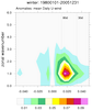
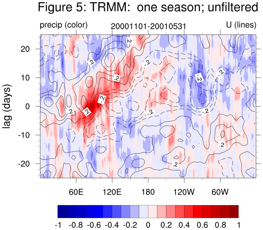
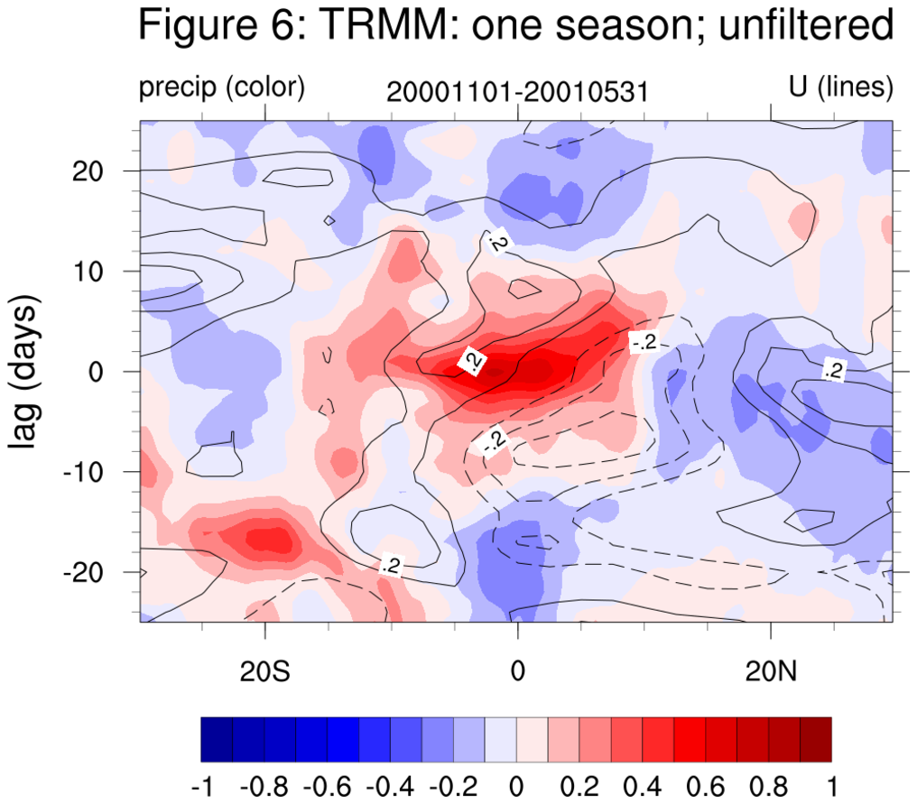
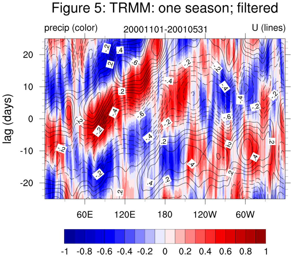
:
For a
specific season [here, winter 2000-2001],
compute a lag correlation diagram using
unfiltered
and
filtered daily data.
The reference time series is the central Indian Ocean regional
precipitation time series
(See
Table 1).
This is correlated with precipitation
and zonal wind anomalies in specified regions at different lags.
Lag-longitude and lag-latitude plots of correlation values for different
regions are shown. Color is for precipitation correlations while
the lagged correlations for the zonal winds are the contours.
These are analogous the Figures 5 and 6 in the reference article except
they are for one season.
The two leftmost are for unfiltered data while the two rightmost
are for 20-100 day band passed filtered data.
The lag-cross-correlations for each season are calculated via the mjo_xcor_lag_season function.
The results are plotted via mjo_xcor_lag_ovly procedure.

 mjoclivar_9.ncl
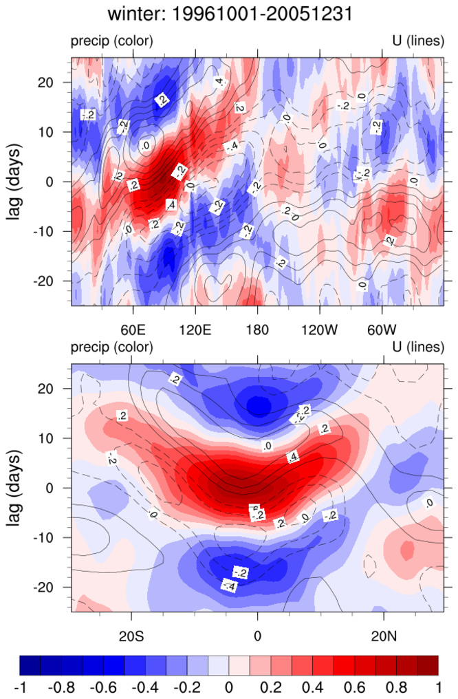
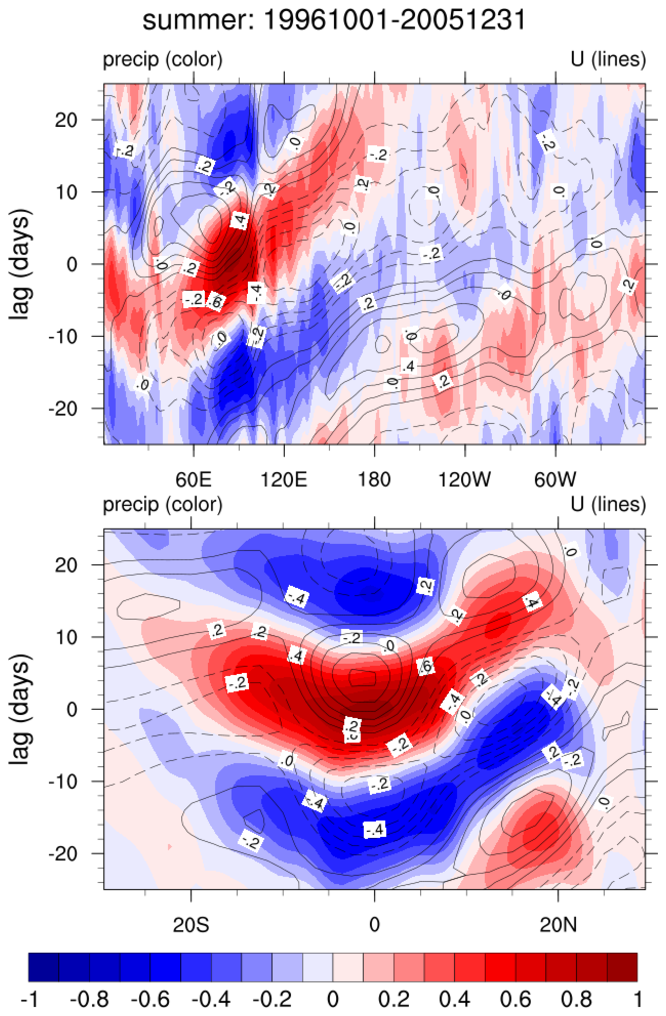
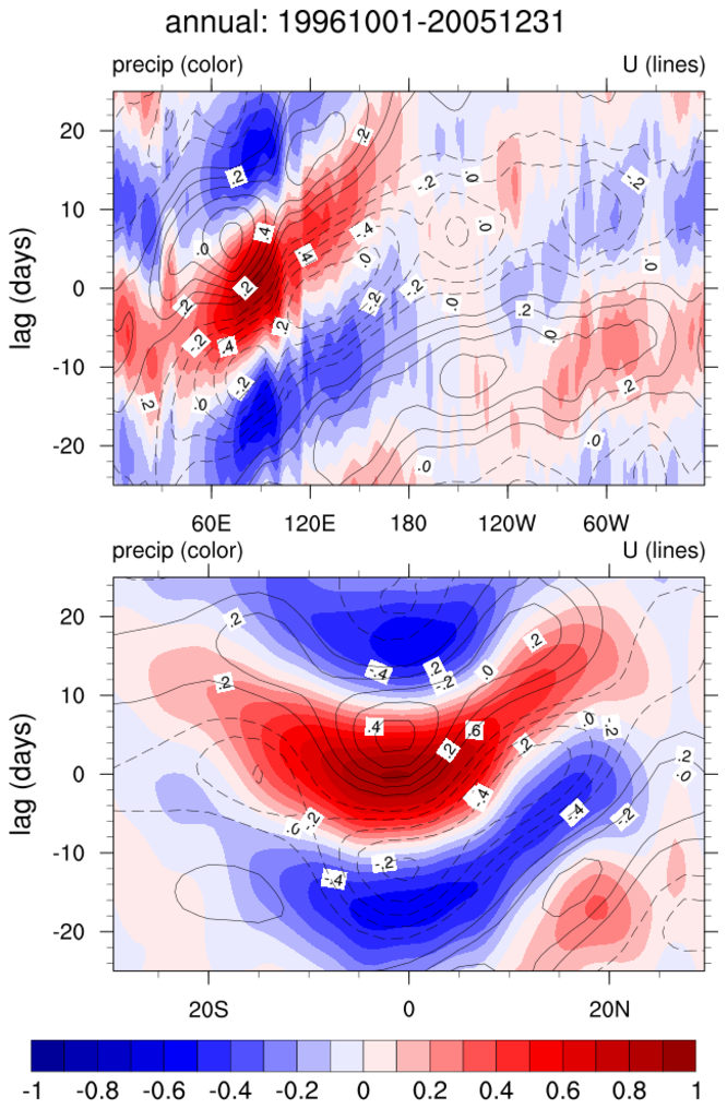
:
Same as
Example 8 except compute the climatological cross correlations
over the period of record using 20-100 band pass filtered data.
The lag-cross-correlations for each season are calculated via the mjo_xcor_lag_season function. Each seasonal cross correlation is averaged by using
the Fischer-z-transform.
The results are plotted via mjo_xcor_lag_ovly_panel procedure.
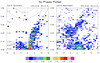
 mjoclivar_10.ncl
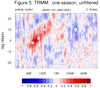
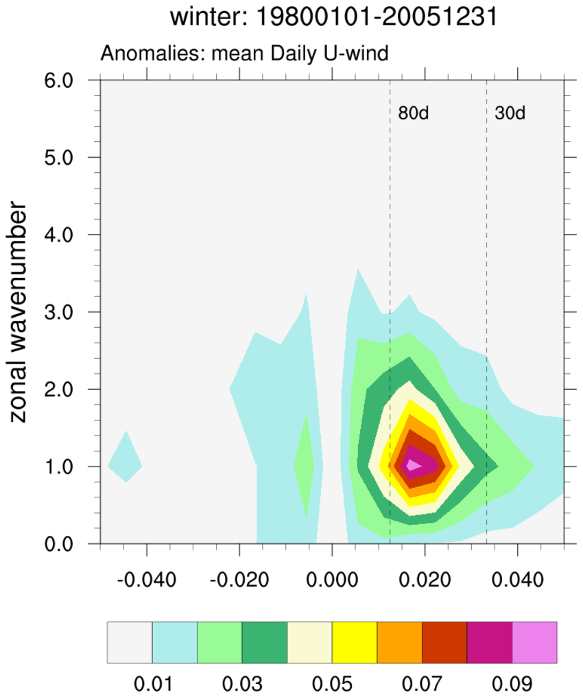
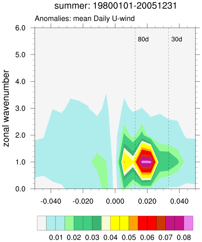
:
The wavenumber - frequency spectra for each season are calculated via the
mjo_wavenum_freq_season function.
The results are plotted via
mjo_wavenum_freq_season_plot procedure.
The vertical
reference lines indicating "day" are drawn for 30 and 80 days (default).
The option "dayLine" (introduced in
v5.1.1) could be used to alter
these. EG: opt@dayLines = (/40,90/) would draw these reference lines
at 40 and 90 days, respectively. The two leftmost figures were generated when the OLR
anomaly file was used. The two rightmost figures were generated when the NCEP
zonal wind [U] anomaly file was used.


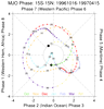
 mjoclivar_11.ncl
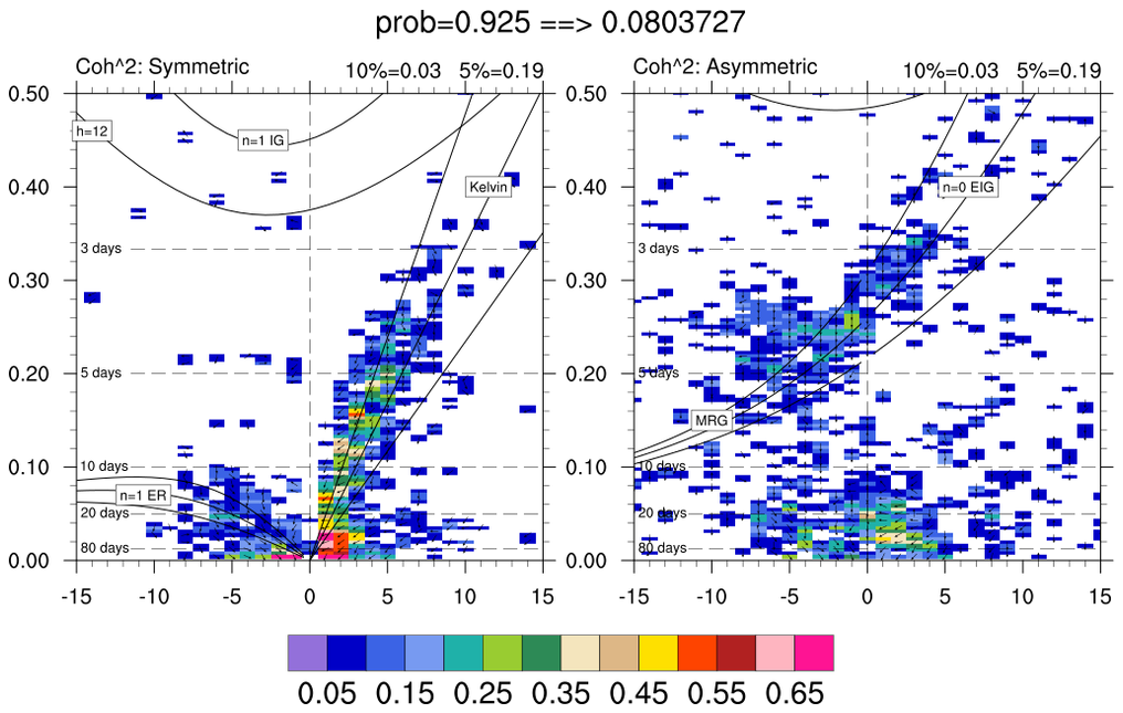
:
Cross-spectra: coherence-squared and phase relationships in wavenumber-frequency space via
mjo_cross function. This is a driver that calls the
mjo_cross function.
The results are plotted via
mjo_cross_plot procedure. The leftmost figure shows
the default plot with both coherence-squared and phase.
The center plot uses the option to plot only where the probability
is greater than 0.925 (not much difference here).
The rightmost plot shows only the coherence-squared with no phases
plotted.
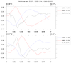
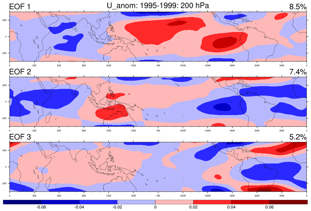
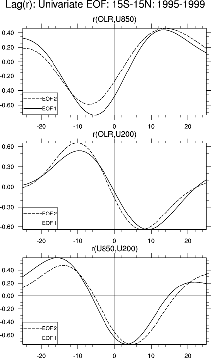
 mjoclivar_13.ncl
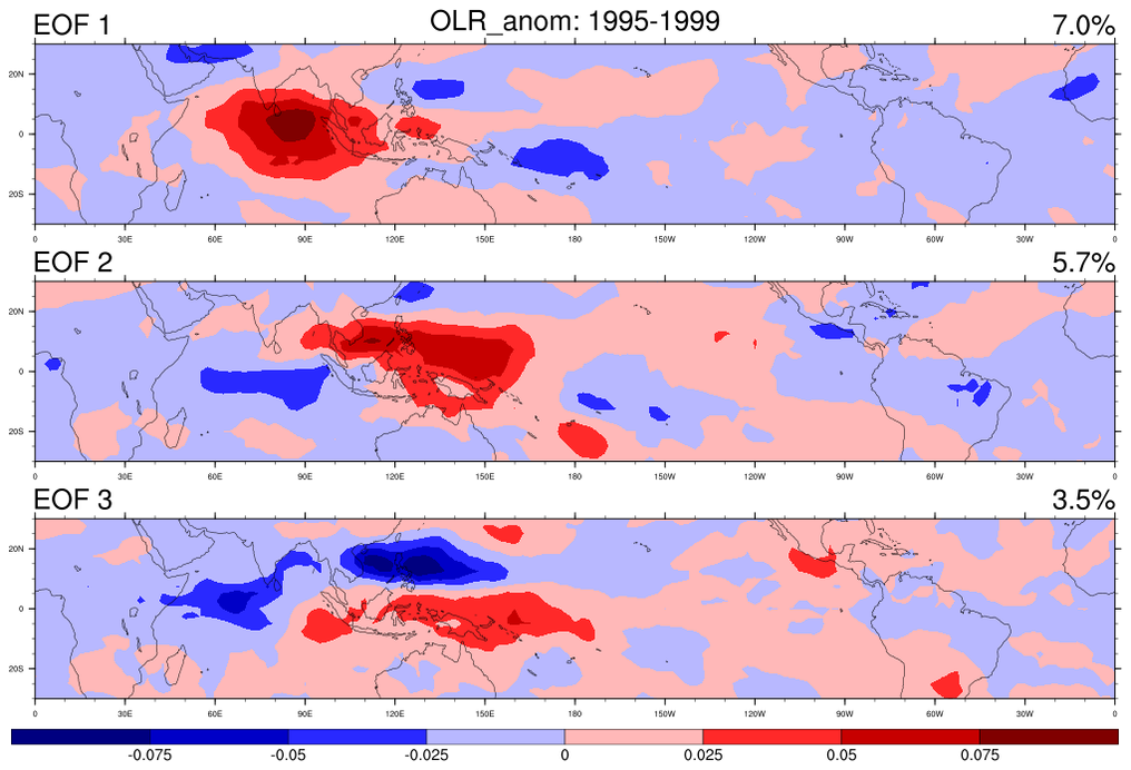
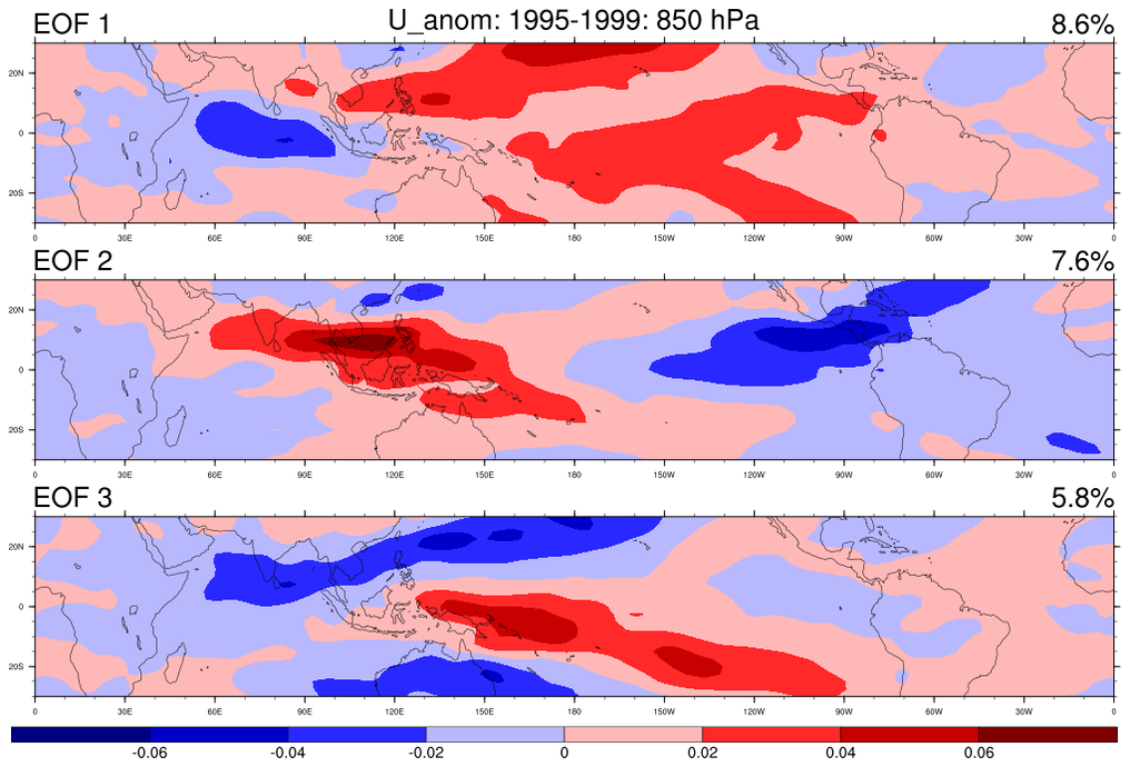
:
Average the 20-100 day band-pass filtered data fields from 15S to 15N;
normalize each of the averaged fields by the square-root of the zonal
mean of their temporal variance; then perform a conventional univariate
EOF analysis.
The left figure shows the (spatial) longitude pattern for EOFs 1 and 2.
The right figure show lag (+/- 25 day) correlations
between EOF 1 and 2 time series for each variable.
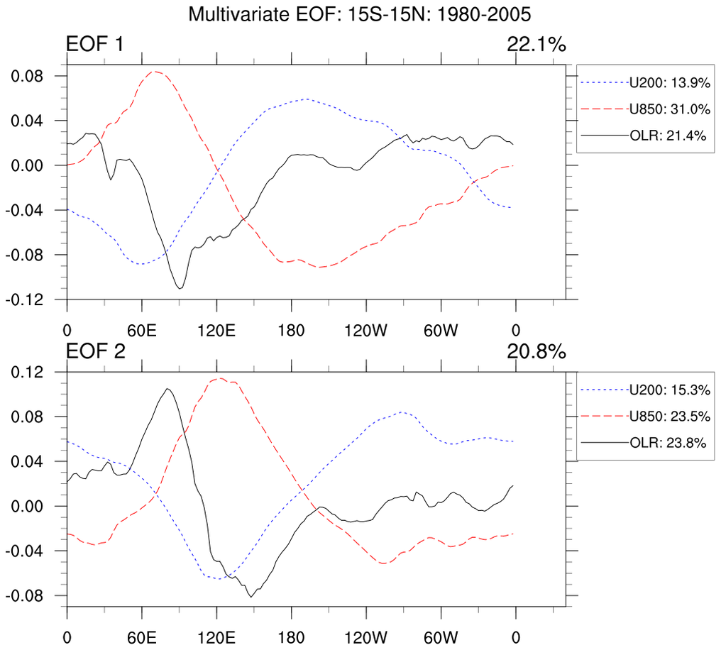
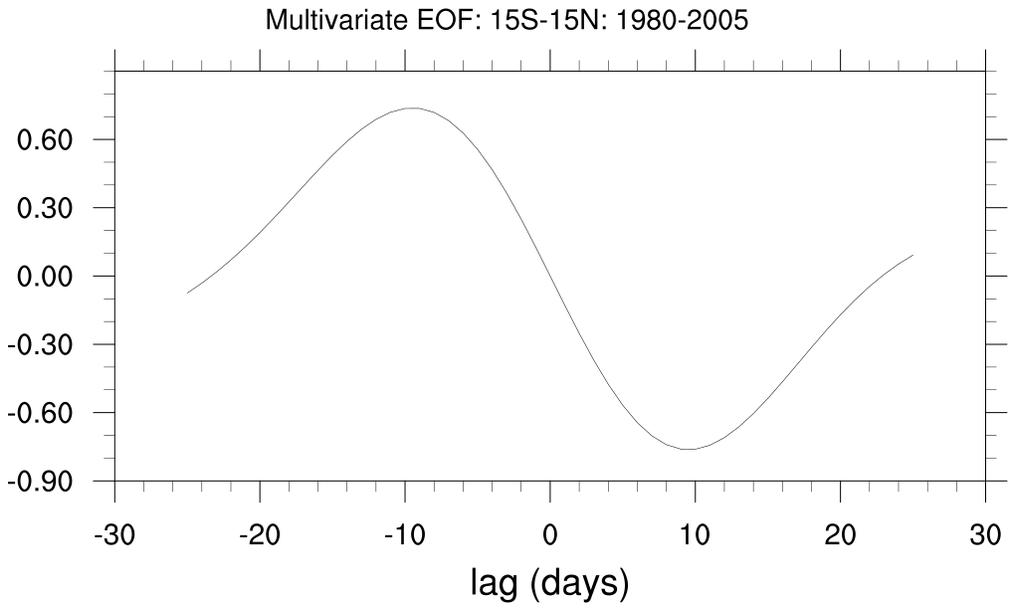
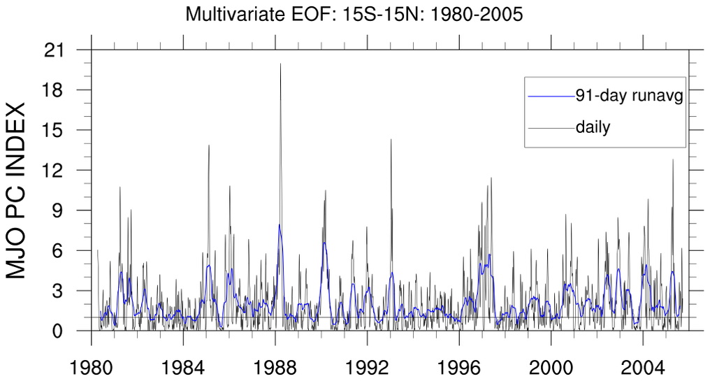
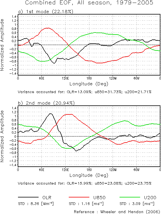
 mjoclivar_14.ncl
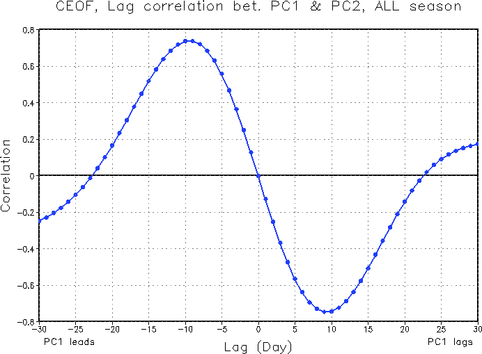
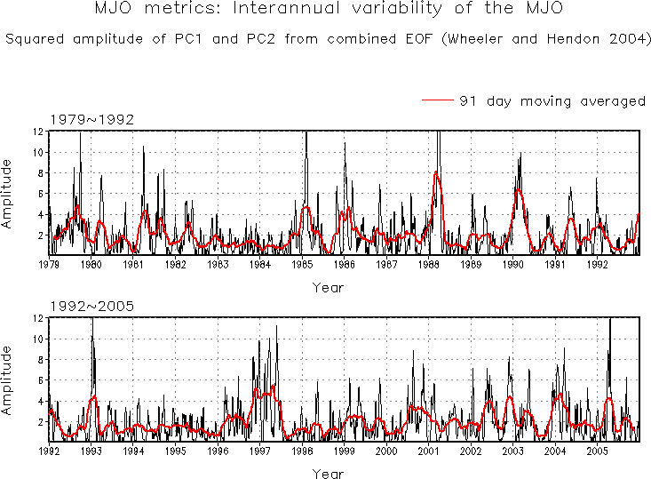
:
Multivariate (Combined) EOF; cross-correlations between EOF1 and EOF2;
time-series of (PC1^2 + PC2^2) and 91-day running mean.
This script was updated 2 March 2015.
Marcus N. Morgan (Florida Institute of Technology) submitted the code segment that calculates the
percent variance for each component in the multivariate EOF.
This script was updated 29 July 2016.
Eun-Pa Lim: Bureau of Meteorology, Australis
For comparison, the equivalent 3 plots from the
Korean MJO-Diagnostics are
(a) eof_all;
(b) lag_all
(c) time series
.
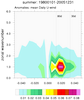
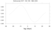
 mjoclivar_15.ncl
:
Read the simple netCDF file created in the previous example and
plot a phase space diagram for a specified time period.
Each month is indicated by a separate line color.
The numbers correspond to the day of the month. The 'nice' plot
is typical of very active MJO periods.
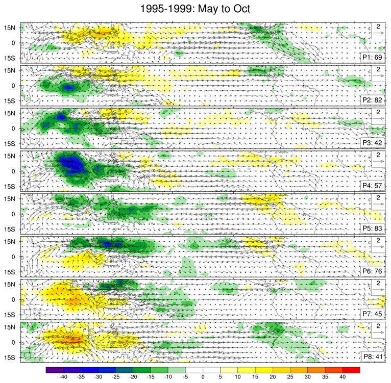
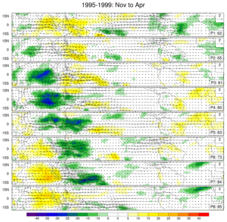
 mjoclivar_16.ncl
:
Create composite life cycles. This example uses 20-100 day
band passed filtered anomaly OLR, U850, V850 for the
years 1995-1999. The netCF file created in
Example 14, which contains the PC1 and PC2, is used
to derive the appropriate MJO phase category.
The size of the reference anomaly wind vector is in
the upper right. The phase (
eg P3, means "Phase 3")
and the number of days used to create
the composite are at the lower right.
This script was updated 29 July 2016. (Source: Eun-Pa Lim, Bureau of Meteorology, Australia)


