NCL Home>
Application examples>
Non-uniform grids ||
Data files for some examples
Example pages containing:
tips |
resources |
functions/procedures
NCL Graphics: Contouring one-dimensional X, Y, Z (random) data
If you have X, Y, Z data represented by one-dimensional (1D) arrays of
the same length, then NCL will contour this data by first generating a
triangular mesh of the data under the hood, and then contouring the
triangular mesh. You can also choose to regrid or interpolate
your data to a 2D grid before plotting.
Here are the options for contouring 1D data:
- Set the sfXArray and
sfYArray resources to the X
and Y arrays respectively, and pass the 1D Z data to the
appropriate gsn_csm contouring routine.
- If your X/Y arrays are lon/lat arrays, then in NCL V6.4.0 and
later you can attach the special "lat1d" / "lon1d" attributes to your
data variable to be plotted. This effectively causes the
sfXArray and
sfYArray resources to
be set for you under the hood.
See the "Plotting data on map"
examples page for more information.
- If you have arrays representing polygons that surround each data point,
then you can additionally set sfXCellBounds and
sfYCellBounds to these arrays for a
(potentially) better plot.
- You can first regrid or interpolate the data to
a rectilinear,
or curvilinear grid using
ESMF regridding, or functions like
like cssgrid, natgrid
and triple2grid.
See the "Random to Grid" examples page.
In all cases, the quality of the resulting plot will be a
function of the distribution of the X and Y arrays, the number of
sampling points, and the 'shape' of the data be contoured.

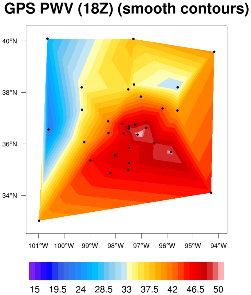
 contour1d_1.ncl
 /
contour1d_old_1.ncl:
The data file for this example
is
pw.dat, which contains
a column of data values, each with a corresponding lat, lon value.
To contour this data correctly over a map, this script attaches the 1D
lat/lon arrays to the data using special "lat1d" and "lon1d"
attributes. As of NCL V6.4.0, the gsn_csm_xxxxx_map scripts
will look for these special attributes in order to correctly plot the
data over a map.
If you have an older version of NCL that doesn't recognize the
lat1d/lon1d attributes, then see
the contour1d_old_1.ncl
script, which sets the sfYArray
and sfXArray resources to these
lat/lon arrays respectively. NCL will internally use the triangular
mesh capability to contour this data.
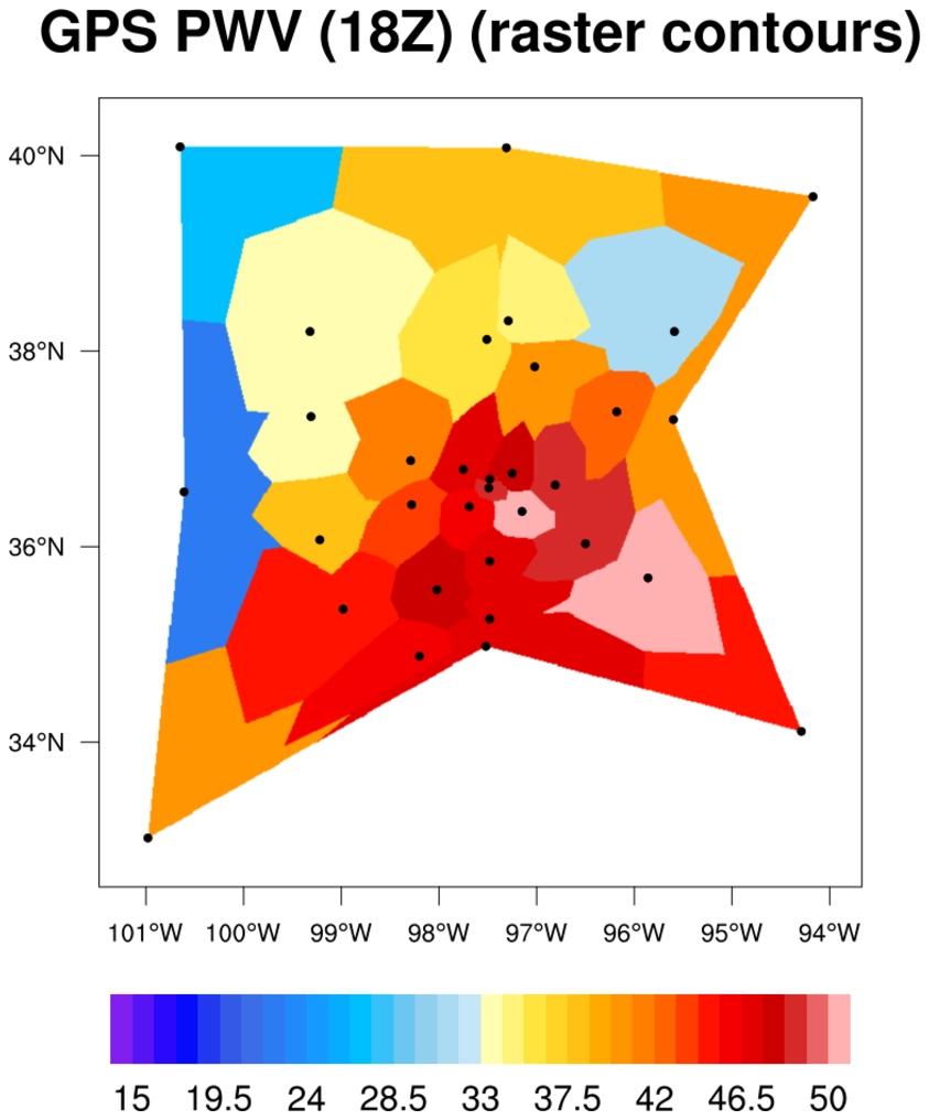
By default, NCL will generate smoothed contours (see first frame)
in an area enclosed by a
convex hull of
the data. If cnFillMode is set to
"RasterFill" (see second frame), then no smoothing will take effect,
but you may get a blocky look. Raster fill can be significantly
faster, but looks smoother if you have more points.
If you have data with concave boundaries, then you may get a
"streaking effect" where NCL is trying to fill areas just outside the
concave boundary area. This is because the contouring algorithm has no
way of knowing where the boundary actually is, and thus creates the
appearance of drawing outside the lines.
In order to hide the streaking effect, you can either
provide "bounds" for each data value via the
sfXCellBounds and
sfYCellBounds resources (see
the Geodesic examples page) or you can
use masking effects to hide streaking areas. See examples mask_8.ncl
and mask_11.ncl on the
Masking examples page.
See example 1 on the "Plotting station
data" page for a similar example using the same data.
 contour1d_2.ncl
 /
contour1d_2_640.ncl:
This example shows how to contour an ARPEGE grid, which came
to us from Christophe Cassou of Meteo-France.
The data for this example are spread across two NetCDF files. The
resolution is pretty fine, so raster contours
(cnFillMode = "RasterFill") are
used.
In the contour1d_2.ncl script,
lat/lon information is provided by setting the
resources sfXArray
and sfYArray. In the
contour1d_2_640.ncl
script, the special lat1d/lon1d attributes are used.
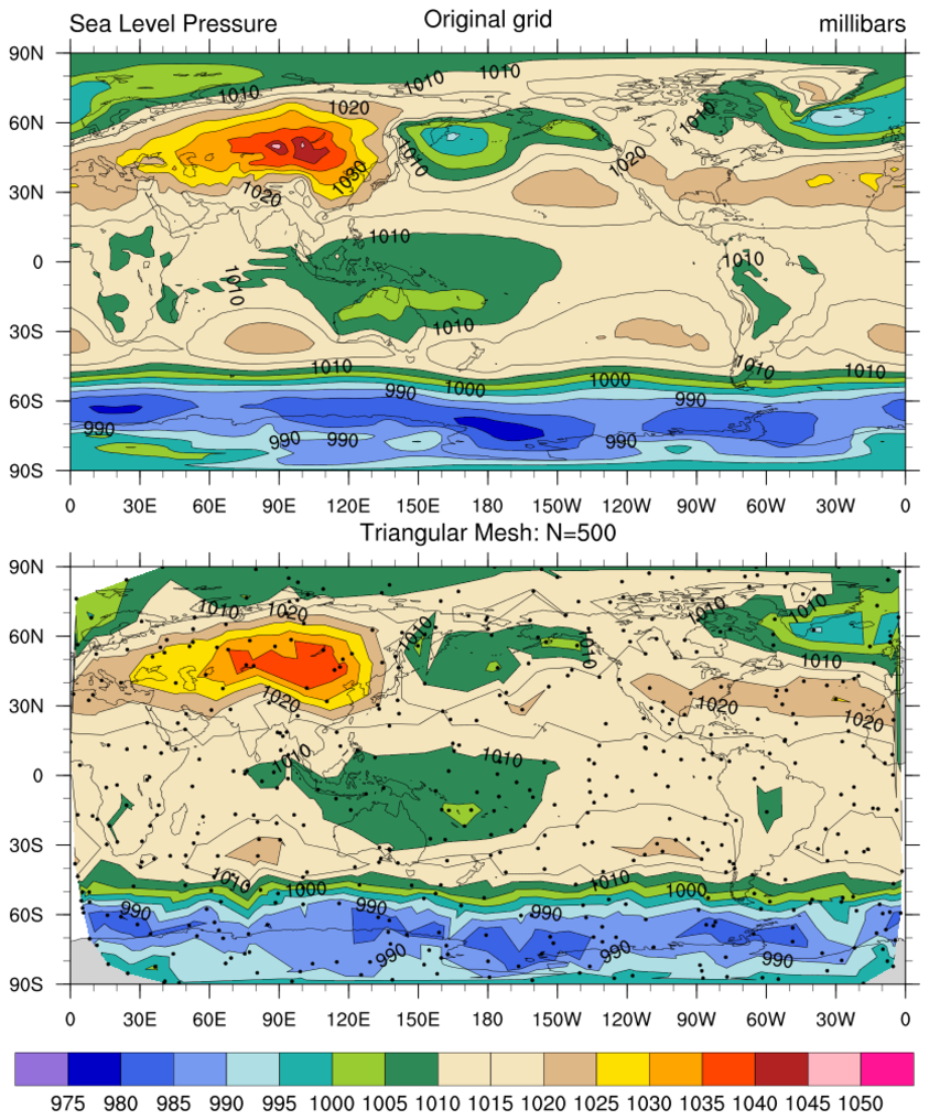
 contour1d_3.ncl
 /
contour1d_3_640.ncl:
Gridded sea level pressures are read; then, for demonstration
purposes,
NOBS are randomly sampled from the grid using
generate_unique_indices
or
random_uniform and small random location
perturbations are added.
The resulting lat[*], lon[*], Z[*] arrays are then contoured using
the sfYArray
and sfXArray resources in the
contour1d_3.ncl script, and
lat1d/lon1d attributes in
contour1d_3_640.ncl.
In this example,
the trGridType
resource is explicitly set to "TriangularMesh". However,
as noted above, this is not necessary.
Note: The input data are on a global grid. Hence, the data are cyclic
in longitude. The resulting plot clearly shows [left and right edges]
that the "TriangularMesh" is not capable of handling this situation.
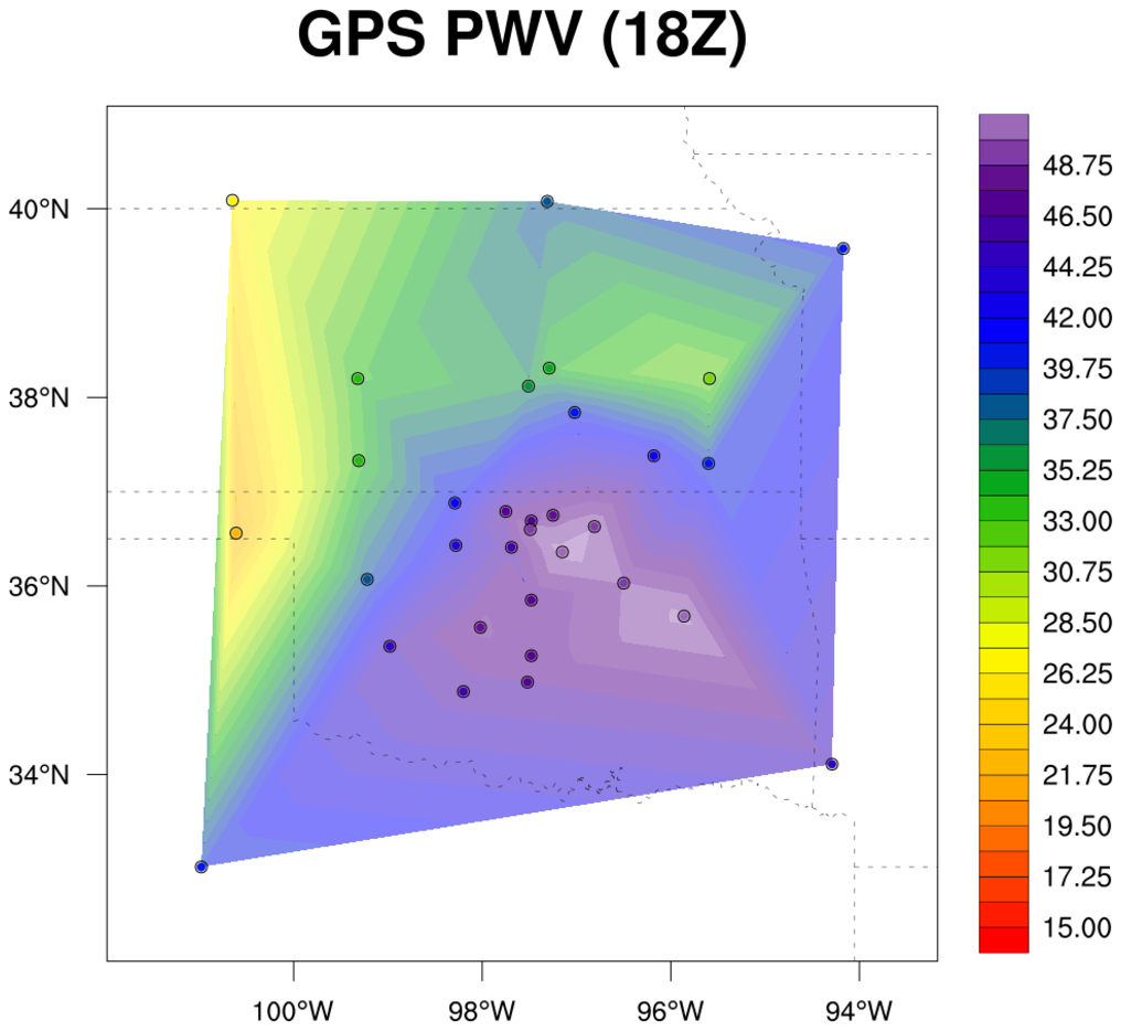
 contour1d_4.ncl
 /
contour1d_4_640.ncl:
This example is very similar to the first one on this page, except the
markers are colored according to the labelbar generated by the color
contours.
The color contours are made more transparent by
setting cnFillOpacityF to 0.5
(default is 1.0). The main purpose of this example is to show how to
color the markers based on an existing contour field.
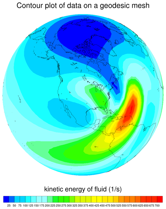
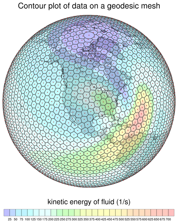
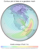 geodesic_1.ncl
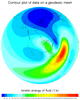
:
sfXArray and
sfYArray are set
to the model's grid center lat/lon arrays (converted to degrees),and
sfXCellBounds
and
sfYCellBounds are set the model's
grid corner lat/lon arrays (also converted to degrees).
The second image shows the structure of a GEODESIC grid, along with its
cell centers.

