NCL Graphics: Overlay Plots

overlay_1.ncl: Create individual plots with gsn_csm_contour_map and gsn_csm_contour, and use overlay to combine them.

As we only wish that the overlaid plot be drawn, gsnDraw and gsnFrame are both set to False in the two resource lists. After overlay is called, draw is called to draw plot, which has had plot_ov overlaid on it. Finally, the frame is advanced, in essence completing the page.

Note that you are not allowed to use any gsn_csm_*_map plotting functions to create the 2nd input in overlay, as an error message will result.

A Python version of this projection is available here.

overlay_2.ncl: Similar to example 1, except gsn_csm_contour_map_overlay is used in lieu of overlay.

overlay_3.ncl: Similar to examples 1 and 2, except here plot2 is manually drawn on plot by not advancing the frame upon the creation of plot.

Note that when manually overlaying, one strives to create each plot the exact same size in the exact same location on the page. In this example, that was trivial. In some cases, the vpXF, vpYF, vpWidthF, and vpHeightF resources, various titles and font heights all need to be set the same for both plots.

overlay_4.ncl: Manually overlay 2 histograms.

To get both histograms to be drawn the exact same size and the same, gsnHistogramClassIntervals and trYMaxF needed to be set the same for both plots.

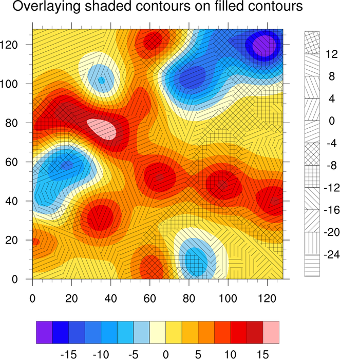
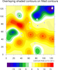
overlay_5.ncl: Documents how to use gsn_contour_shade to create an overlay plot that is then overlaid on the base plot by using overlay.

This is one way to overlay a pattern filled contour field on top of a different color filled contour field. Another way can be found on example 14 on the Contour Effects applications page.

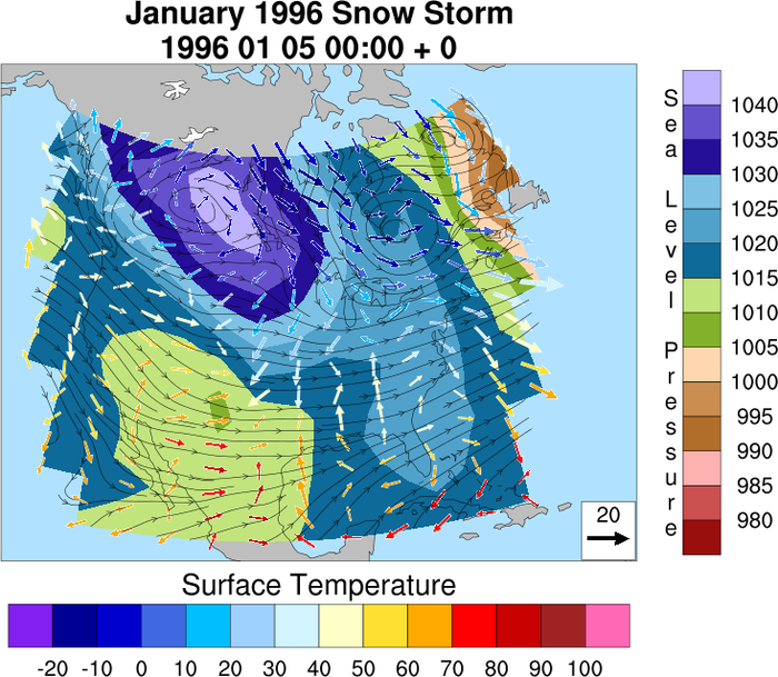
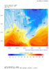
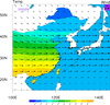
overlay_6.ncl: Demonstrates how to overlay a color filled contour field, streamlines, and color filled vectors all on one plot.

Two label bars are created, one for the color filled contour field, and one for the color filled vector field. Individually 4 plots are created: A plot showing just a map, a color filled contour field plot, a streamline plot, and a color filled vector plot. overlay is then used to overlay the contour, streamline and vector plot on the map plot.

The resources cnFillPalette and vcLevelPalette are used to indivudally assign color maps for the color contours and vectors.

A Python version of this projection is available here.

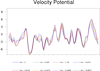
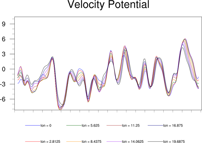
overlay_7.ncl: Documents how to overlay xy plots whose timeseries are of different sizes. As gsn_csm_xy expects each input timeseries to be the same size, this is one method that can be used to add timeseries of different lengths to a single plot.

gsn_add_annotation is used to add a legend to the overlaid plot, which allows the legend to be resized if the plot itself is resized.

conOncon_5.ncl: "Spaghetti" contours overlaid on a map. The first spaghetti contour is created using gsn_csm_contour_map, and subsequent contours are created using gsn_csm_contour.

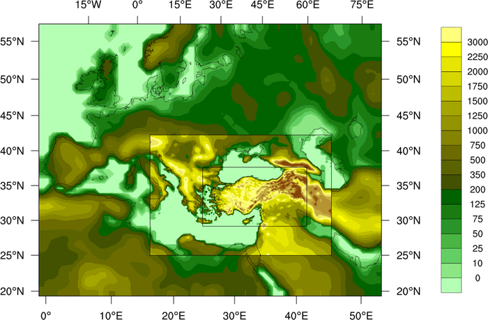
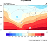
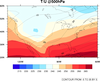
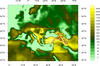
conOncon_9.ncl: This image describes land use in different resolutions for each domain. This script was originally written in PyNGL by Ufuk Utku Turuncoglu of the Istanbul Technical University in relation to a Turkey Climate Change Scenarios project.

The overlay procedure is used to do the multiple contour overlays. These contours are over a map, so the first contour (coarse) plot is created with gsn_csm_contour_map, and the other two contour plots are created using gsn_csm_contour.

Polylines are drawn on top of the map to show the three domains.

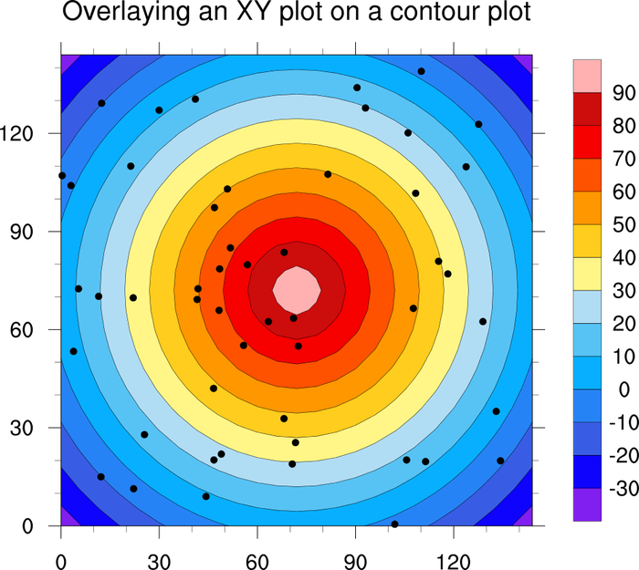
overlay_8.ncl: Shows how to overlay a scatter plot on a contour plot. The key is that the axes of both plots must be in the same data space.

The next example shows how to overlay two plots that are not in the same data space.

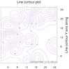
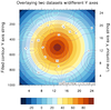
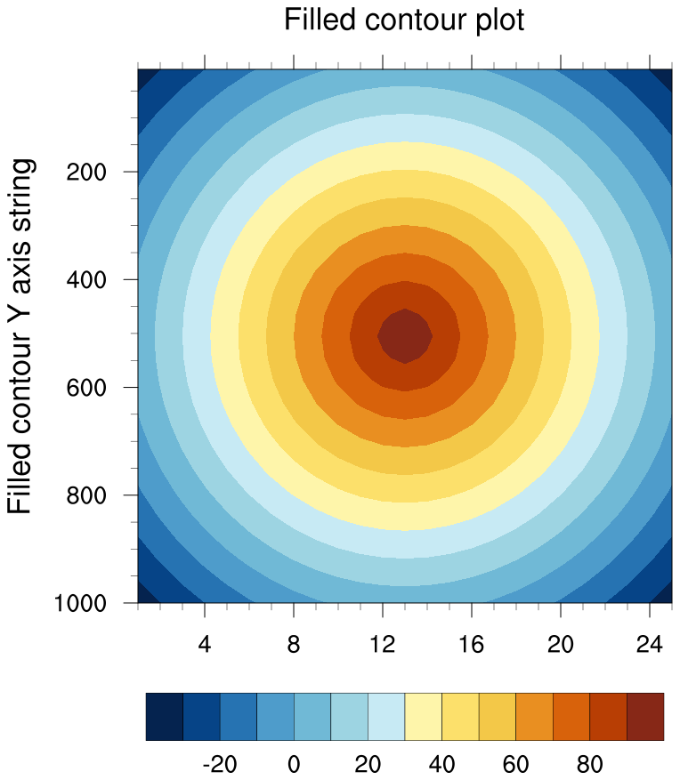
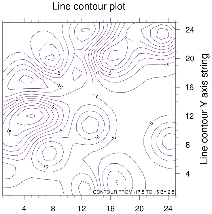
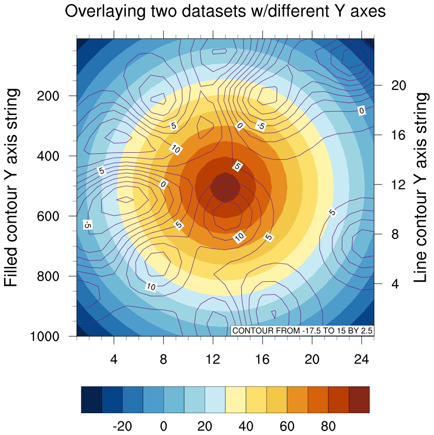
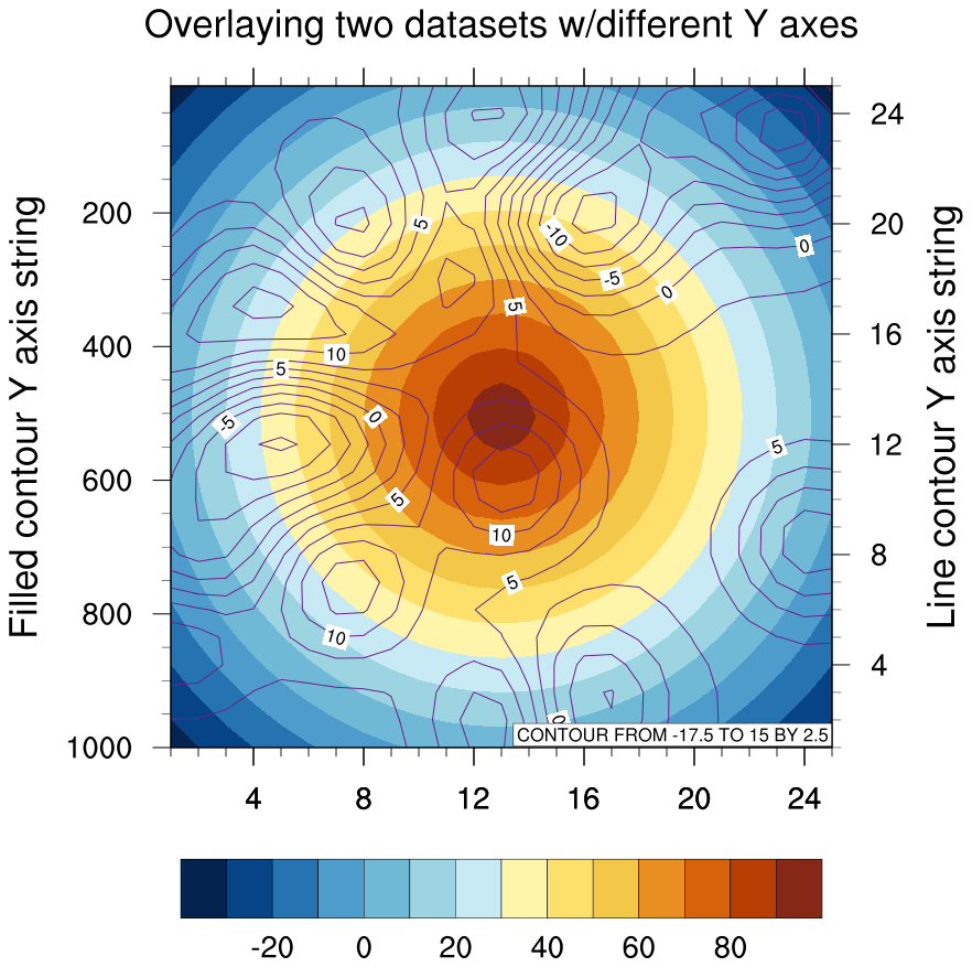
overlay_9.ncl / overlay_9a.ncl: Shows two different ways to overlay a line contour plot on a filled contour plot when they have two different axes. The "overlay_9.ncl" script uses gsn_add_annotation to add the line contour plot as an annotation of the filled contour plot. The "overlay_9a.ncl" script uses overlay procedure, along with setting the special tfDoNDCOverlay resource to True.

Note that the left axis corresponds with the filled contour plot, and the right Y axes with the line contour plot.

Since the axes are not in the same data space, this example only works if the Y ranges of the two plots line up exactly.

When you use overlay, the tickmarks and labels get removed from the overlay plot. The "overlay_9a.ncl" example adds them to the base plot on the Y right axis.

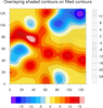overlay_10.ncl: Shows how to overlay a shaded contour plot on a filled contour plot and get labelbars for both plots by drawing one vertically and one horizontally.

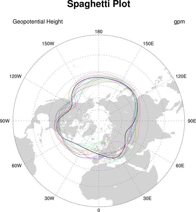
xy_32.ncl: This example shows how to draw a 8-curve XY plot with 4 legends stacked side-by-side.

In order to do this, it is necessary to create 4 XY plots, each with two curves and two items in its legend. The legend for each plot is moved to the right or left slightly so they don't overlap. The plots are then all "connected" into one plot using the overlay procedure.

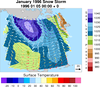
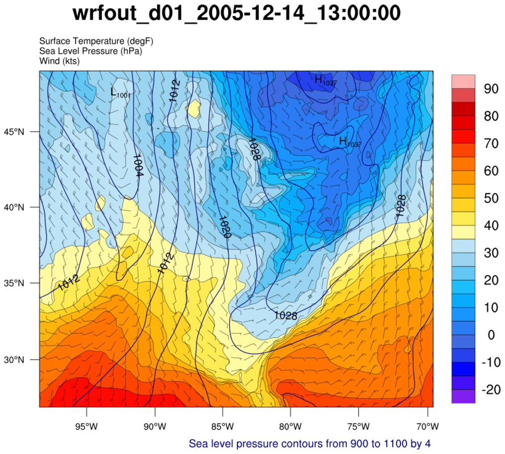
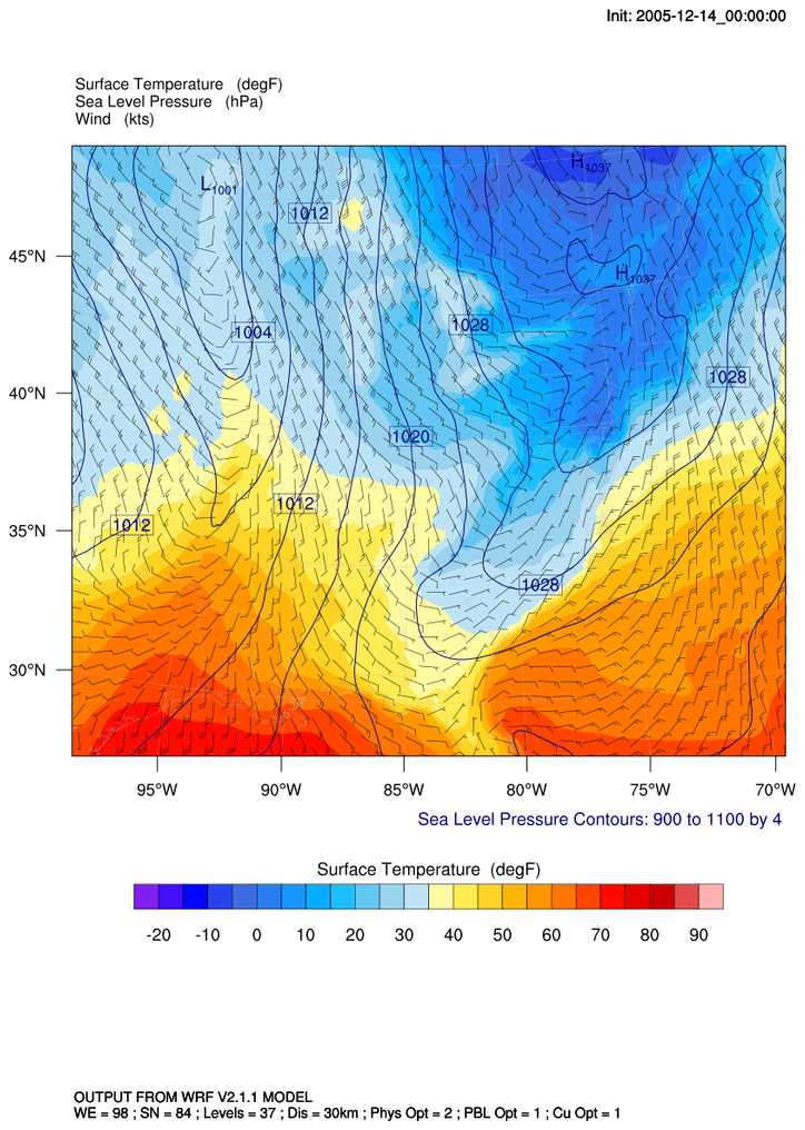
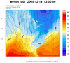wrf_gsn_5.ncl This example shows how to overlay line contours, vectors, and filled contours on a map. The data and map projection are all read off a WRF output file.

wrf_nogsn_5.ncl This example is similar to the previous one, except it shows how to use WRF plotting functions instead of gsn_csm plotting functions.

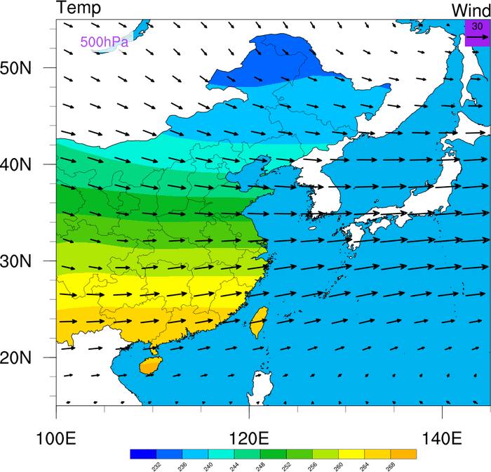
overlay_11.ncl: This example shows how to overlay vectors on top of a filled contour plot, where the contours are masked by a geographical area and the vectors are not. The masking is accomplished by setting:

  mpres@mpDataBaseVersion   = "MediumRes"
  mpres@mpMaskAreaSpecifiers = (/"China:states","Taiwan"/)

The mask area specifier names are part of the predefined group names available in the "MediumRes" map database.

This script was written by Yang Zhao (CAMS) (Chinese Academy of Meteorological Sciences).

There are two versions of this projection available in Python. Version (a) is found here and version (b) is found here.

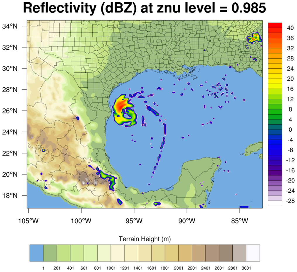
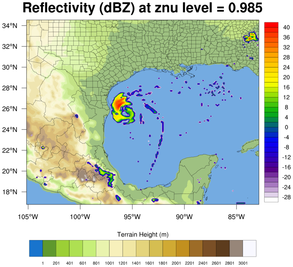
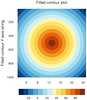
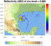
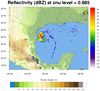
overlay_12.ncl: This example shows how you can create two color contour plots, each with their own color map, and then use the overlay procedure to overlay them into a single image.

The cnFillPalette resource is used to set the color map for both plots. The color map for the reflectivity contours is first read in using read_colormap_file, so that the first color can be set to transparent.

Transparency is used in both plots to subdue the colors in the terrain map, and to make one of the colors in the reflectivity plot completely transparent.

Important note: In NCL V6.3.0 and earlier the labelbar does not reflect the same opacities as the filled contours; this bug was fixed in NCL V6.4.0. A new resource called lbOverrideFillOpacity was introduced in NCL V6.4.0 which allows you to keep the labelbar colors fully opaque independent of the opacity of the filled contours.

The first frame shows the partially opaque labelbar, and the second frame shows a fully opaque labelbar created by setting lbOverrideFillOpacity to True.

For a version of this script that does animation, see newcolor_10.ncl on the RGB/A example page.

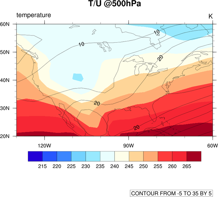
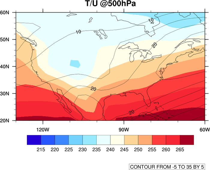
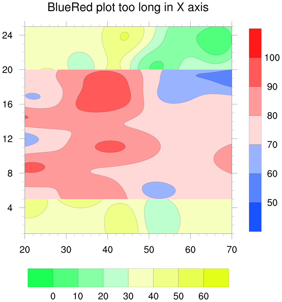
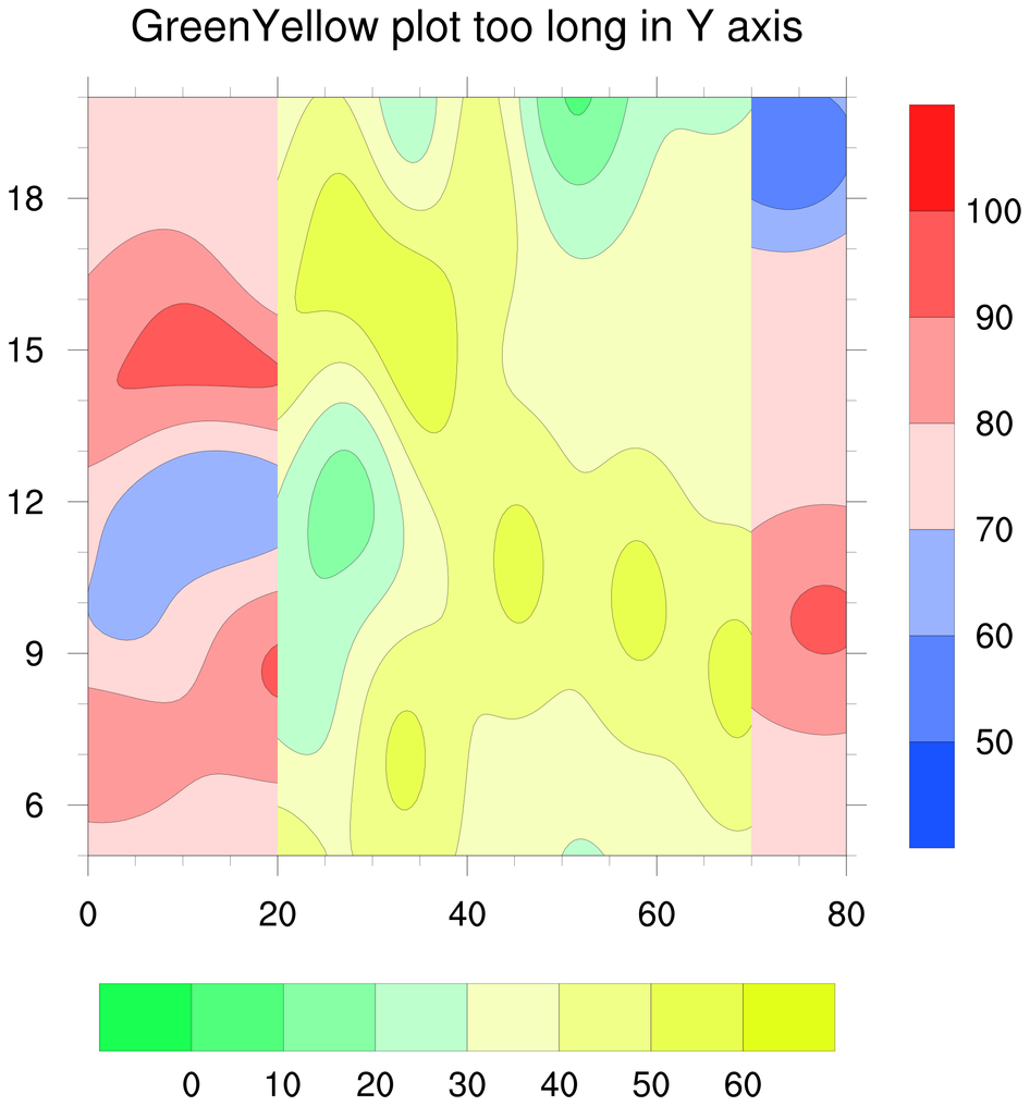
overlay_13.ncl: This example shows what happens when you try to overlay two plots that don't have the same X and Y axis ranges. The X/Y axis from the "base" plot is the one that gets used for both plots, which may cause your "overlay" plot to be cut off if its X and/or Y axis outside the range of the X/Y axis of the "base" plot.

In this example, the X axis of the second plot is longer than the first, and the Y axis of the first plot is longer than the second. The first image shows what happen when you overlay plot #2 on plot #1. The second image shows what happen when you overlay plot #1 on plot #2.

For the third image, the X/Y range was increased to be large enough to accommodate both plots.

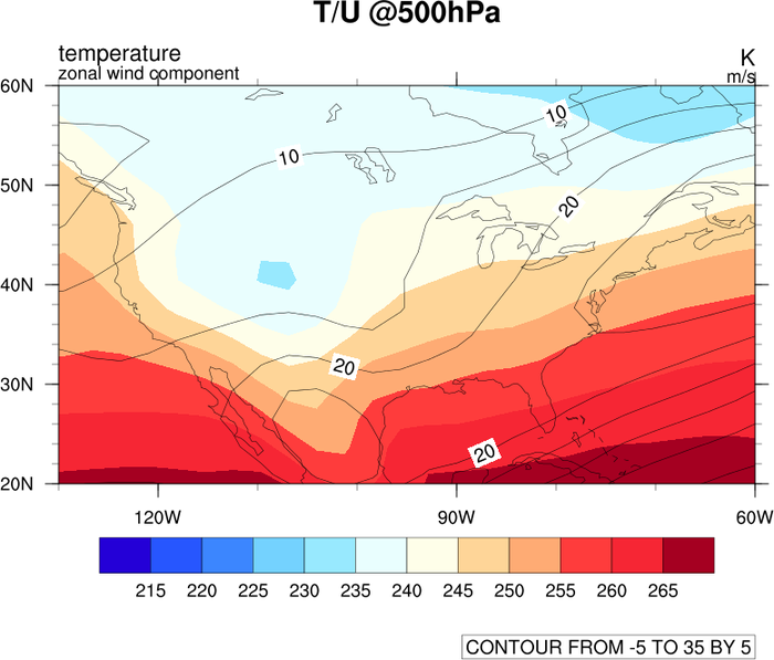
overlay_14.ncl: This example illustrates overlaying an 'xy-object' onto a 'contour-object.' The original source code was from:

  - Ehimen Williams: Institute of Meteorology and Geophysics
  - University of Cologne, Germany

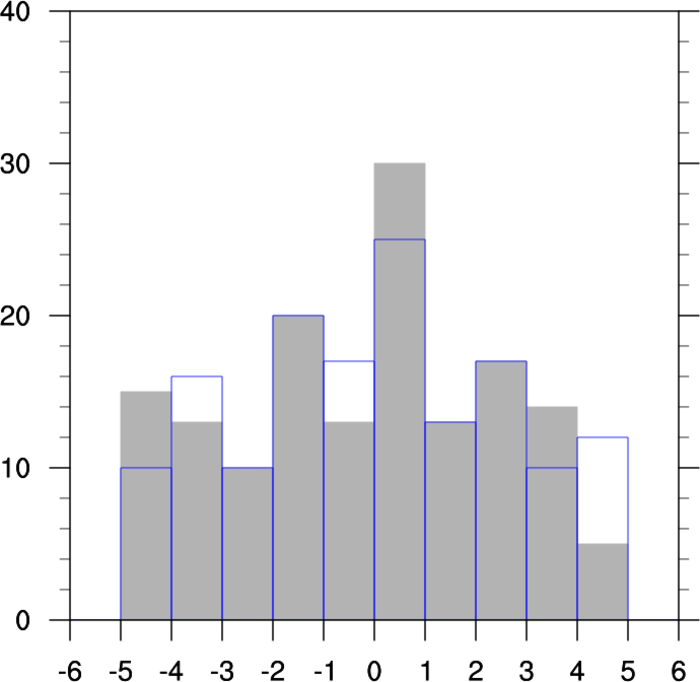
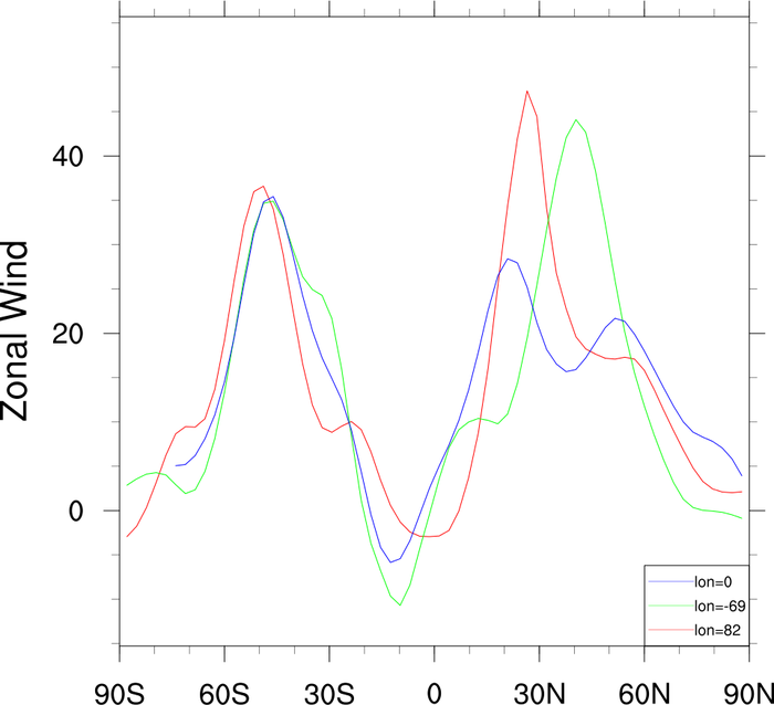
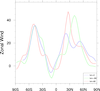
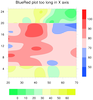
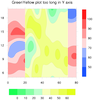
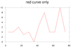
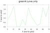
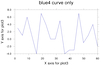
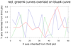
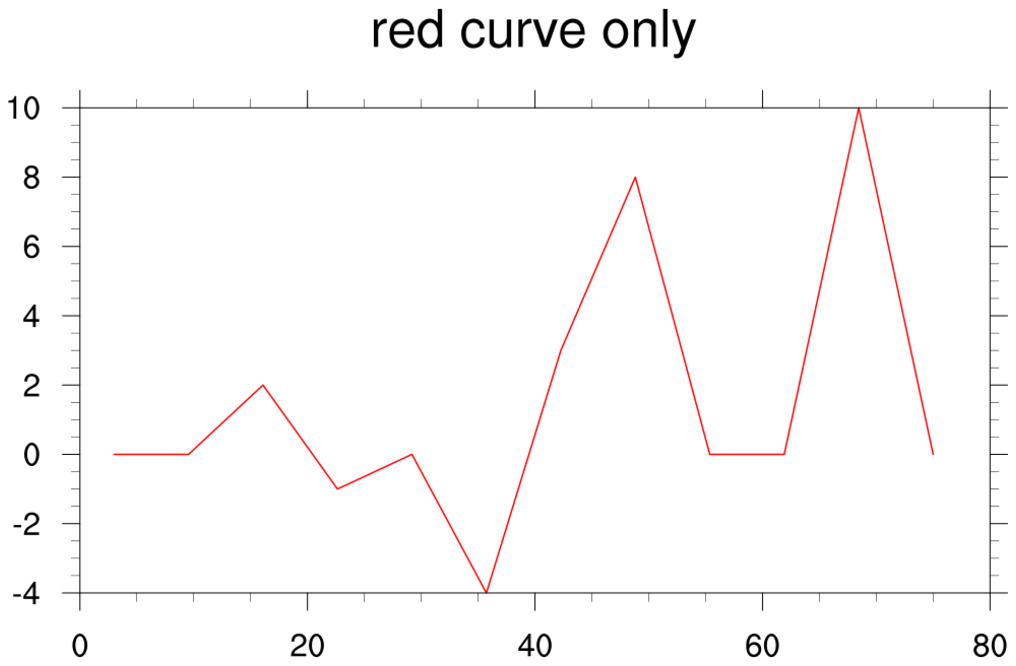
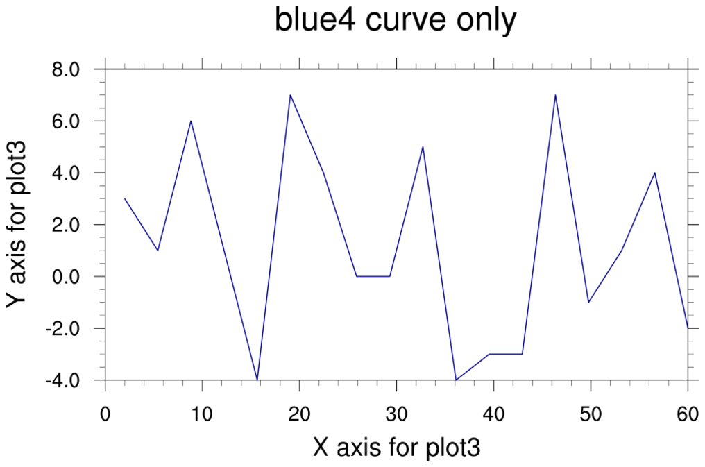
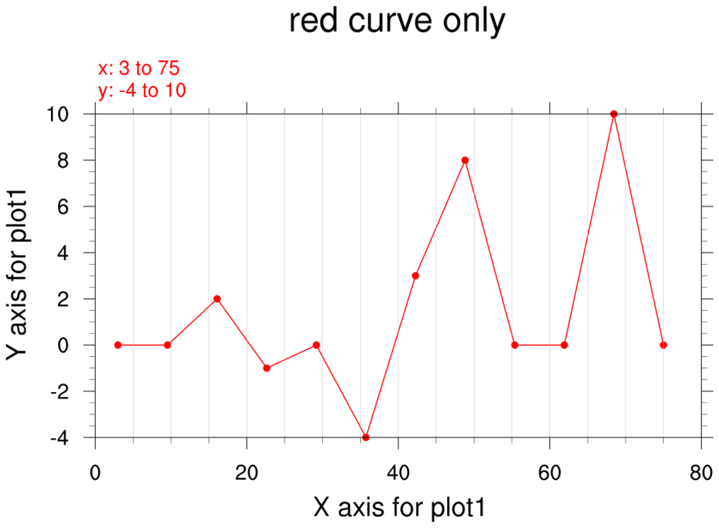
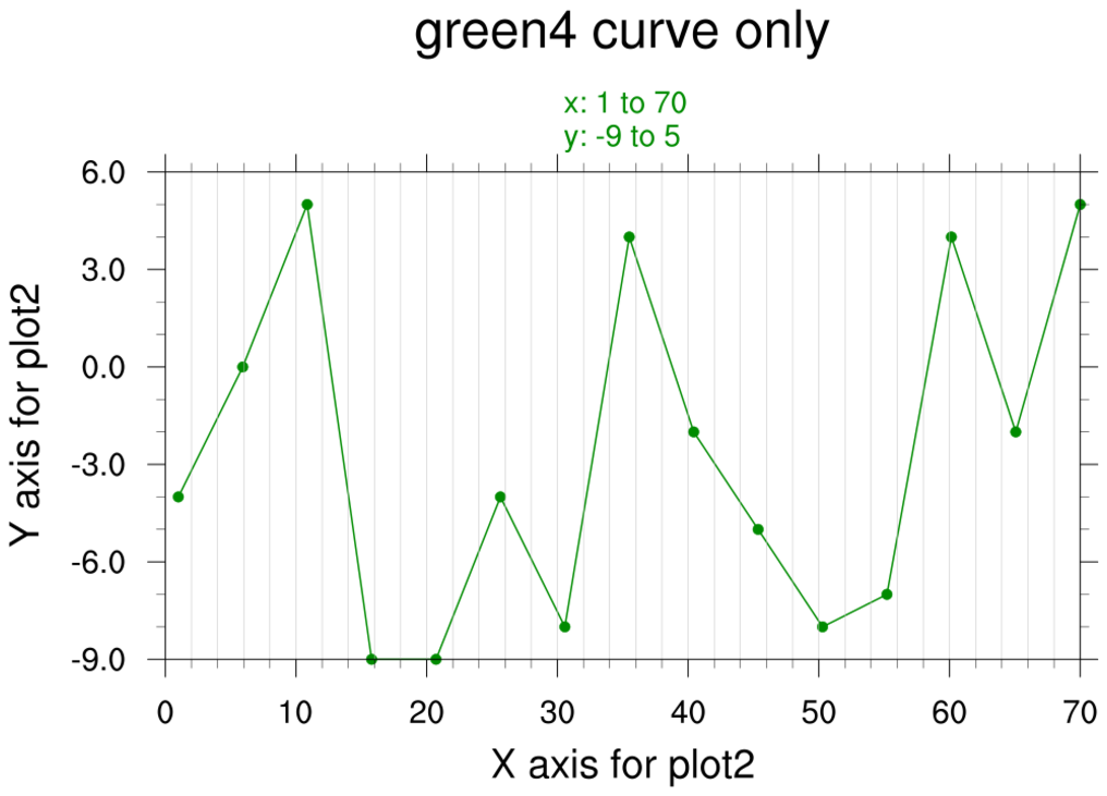
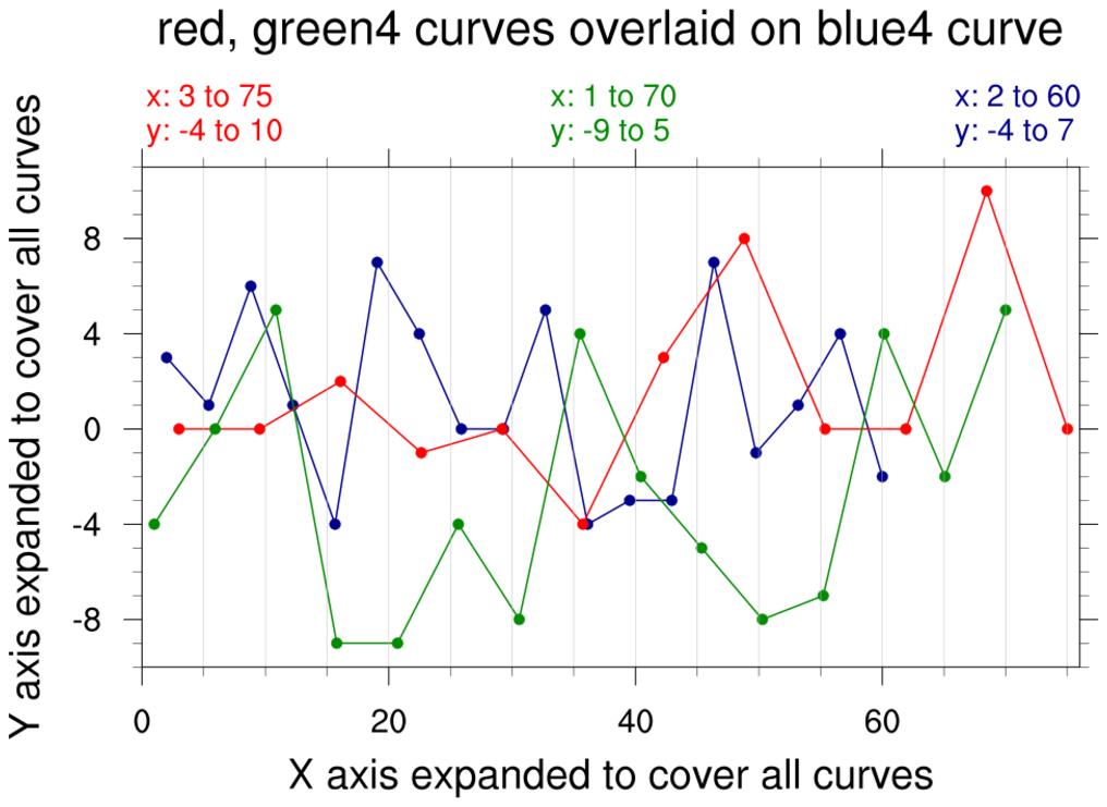
overlay_15.ncl: This example overlays two XY plots on a third XY plot (the base plot). For illustrative purposes, the three individual plots are drawn, and then the fourth image shows the overlaid plots.

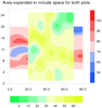
This script shows how the overlay procedure adopts the X/Y axis from the base plot. This means that the overlaid plots may be cut off if their axis ranges are outside the axis ranges of the base plot. The overlaid curves will be plotted correctly, but you will note in the fourth image that the red and green curves are truncated because they don't fit in the same range as the blue curve.

If you want the axes of the base plot to be large enough to encompass all overlaid curves, then you will need to set the resources trXMinF / trXMaxF / trYMinF / trYMaxF. Also note that the main title and the X and Y axis titles from the base plot will be inherited from the base plot. This example uses setvalues to change the titles after the plot is created, but before overlay is called.

For an example that shows how to set the axis ranges and do more customization of titles, see example overlay_16.ncl below.

overlay_16.ncl: This example is similar to overlay_15, but it sets more resources to customize the plot. For example, vertical grid lines were added and the XY curves are drawn with both lines and markers.

When overlaying plots, note that the titles created by gsnLeftString, gsnCenterString, and gsnRightString are retained from the overlaid plots and the base plot, but the tiMainString title is only retained from the base plot.