NCL Home>
Application examples>
Plot techniques ||
Data files for some examples
Example pages containing:
tips |
resources |
functions/procedures
NCL Graphics: Contour Effects
There are numerous examples of contour effects throughout the
Applications page. This page is dedicated
to specialized ways of controlling the look of contours, via shading,
transparency (new in V6.1.0), color fill, line thicknesses, and dashed
patterns.
Three new resources were added in V6.1.0, allowing you to specify a
color palette for filled contours (and whether to span that color
palette), and controlling the opacity of color colors.
In addition, in V6.1.0,
the cnFillColors resource can now
be given an n x 4 array of RGBA values, allowing to specify the
opacity of individual colors.
Three other popular resources and a function include:
This page mentions some older methods for doing shading
and color fill, all of which have been superceded by
gsn_contour_shade:
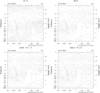
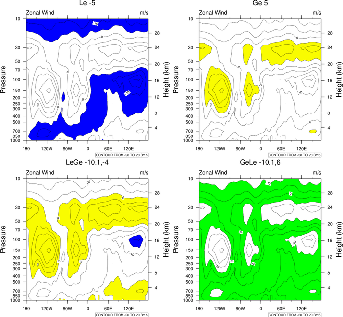
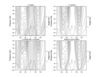 coneff_7.ncl
: A panel plot
demonstrating four ways to selectively shade contour data. All of
these functions require user defined
fill patterns.
The four functions listed below have been superceded by the single
function gsn_contour_shade. (Available in version 4.3.0 and later.)
We recommend you use this instead. See coneff_13 below for a demonstration of how to use
gsn_contour_shade.
ShadeLtContour
ShadeGtContour
ShadeLtGtContour
ShadeGeLeContour
Note! ShadeLtContour,
ShadeGtContour and ShadeLtGtContour all use greater (less)
than, and NOT greater (less) than or equal to. These functions will
find the closest CONTOUR less than the specified threshold value when
choosing when to start shading. This is important to note when the
threshold values are being set in the above functions. For example, if
there are contour levels at (/1.0,1.5,2.0,2.5/), and one wants to
shade all areas greater than 2., ShadeGtContour should be used as such: plot
= ShadeGtContour(plot,2.2,1) ShadeGtContour will select the first
contour less than the given threshold value, in this case it
will select the 2 contour level. Thus, all areas greater than 2. will
be shaded. If instead 2.0 is specified as the threshold value, then
all contours greater than 1.5 and higher will be shaded. This
is because the 1.5 contour is the next contour level less than (and
not equal to) the given threshold value of 2.
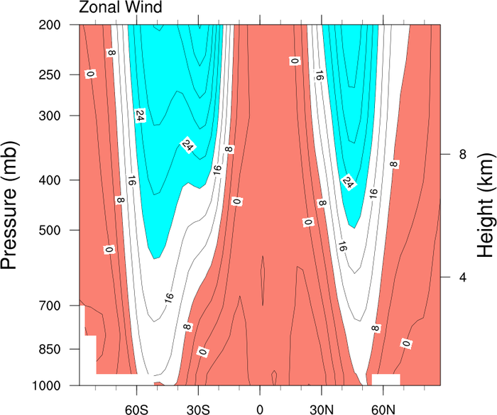
 coneff_9.ncl
: Shows how to take the
function in
example 6 to make a
particular line disappear.
The color "transparent" exists in NCL, so that in this example the line
is draw but colored "invisible".
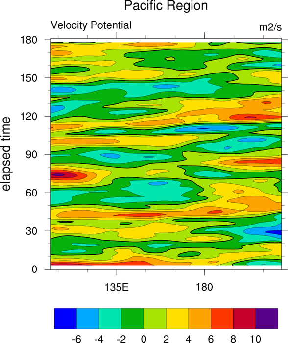
 coneff_10.ncl
: This example
illustrates the use of shadings and hatchings to create a black and
white plot. Actually, only one shading and one hatching pattern are
used but the density of the patterns are altered giving the impression
of several different patterns.
cnFillPatterns is the resource
that will allow the user specify what fill patterns to
use.
 coneff_12.ncl
: This example shows
how to apply a fill pattern and/or fill color to areas with missing
data. It also shows how to turn on the missing value perimeter
line. Note: NCL treats all values set to the attribute _FillValue as
missing values.
When cnFillOn=True, NCL color
fills areas with missing values the backgroud color, in this case
white. This is shown in the top plot.
The middle plot has the missing value perimeter turned on via cnMissingValPerimOn, and the perimeter
line color is set to red using cnMissingValPerimColor. The missing value
fill pattern is set to solid fill (0) using cnMissingValFillPattern, and the missing
value fill color is set to blue using cnMissingValFillColor. Important note:
Even if you just want to fill missing areas with a color as in this
case, you still need to set cnMissingValFillPattern = 0. If you do
not set cnMissingValFillPattern,
the default = -1, and no pattern or color fill will be drawn.
The bottom plot is the result of setting cnMissingValFillPattern
= 5, cnMissingValFillScaleF
= .8 (increase the density of the fill pattern), changing cnMissingValPerimColor
to black, setting the missing value perimiter line to dash using cnMissingValPerimDashPattern,
and increasing the thickness of the missing value perimeter line by
using cnMissingValPerimThicknessF.
For this example, cnFillMode is
set to the default "AreaFill". Not all of the above missing value
resources work with every cnFillMode. For instance, "CellFill" and
"RasterFill" modes do not allow use of cnMissingValFillPattern (= 0 for these
modes). Please consult the cnFillMode documentation for more details
about what missing value resources can be used with each FillMode.
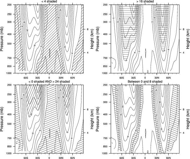
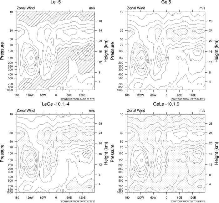
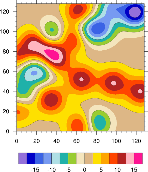
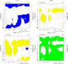 coneff_13.ncl
: In version
4.3.0 a new function
gsn_contour_shade was added that allows you
to add shading and/or color fill between specified contour levels in
your plot. Note that the shading will always begin at a contour,
and not neccesarily at the user specified
gsn_contour_shade input arguments.
Check your plot to make sure that the results are what you expected.
The first frame shows how to do pattern shading four different ways, and the second
frame shows the same thing using solid color fill.
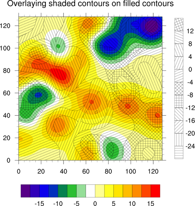
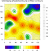 coneff_14.ncl
: Overlay
shaded contours on color-filled contours, and create two
separate labels for each set of contours.
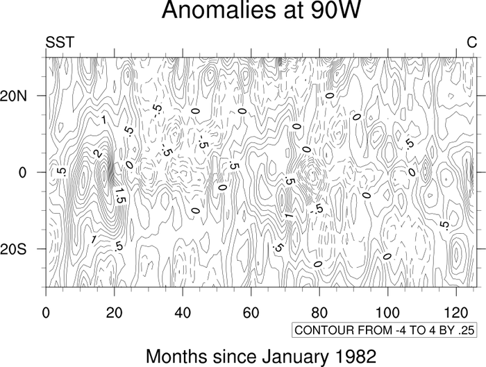
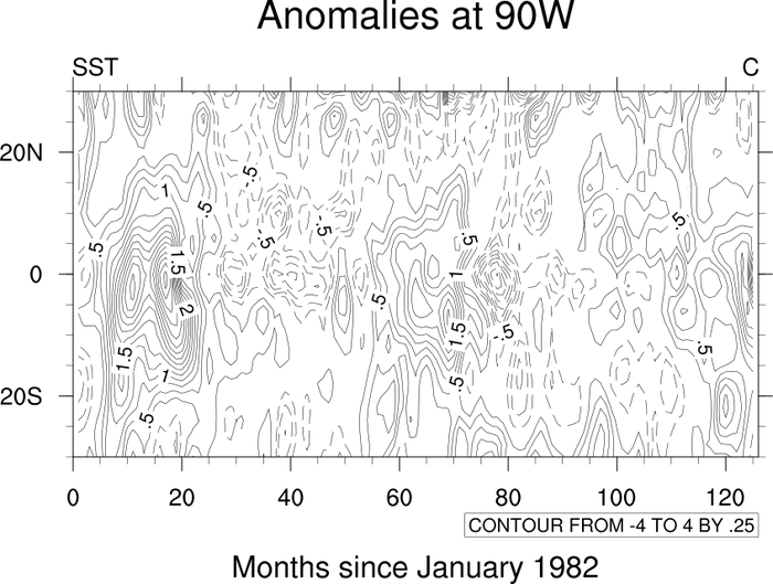
 coneff_15.ncl
: Using the
cnLevelFlags resource to control which
contour lines get drawn. You can set this resource to an array of
strings with the values "NoLine", "LineOnly", "LabelOnly", or
"LineAndLabel".
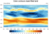
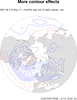
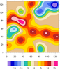
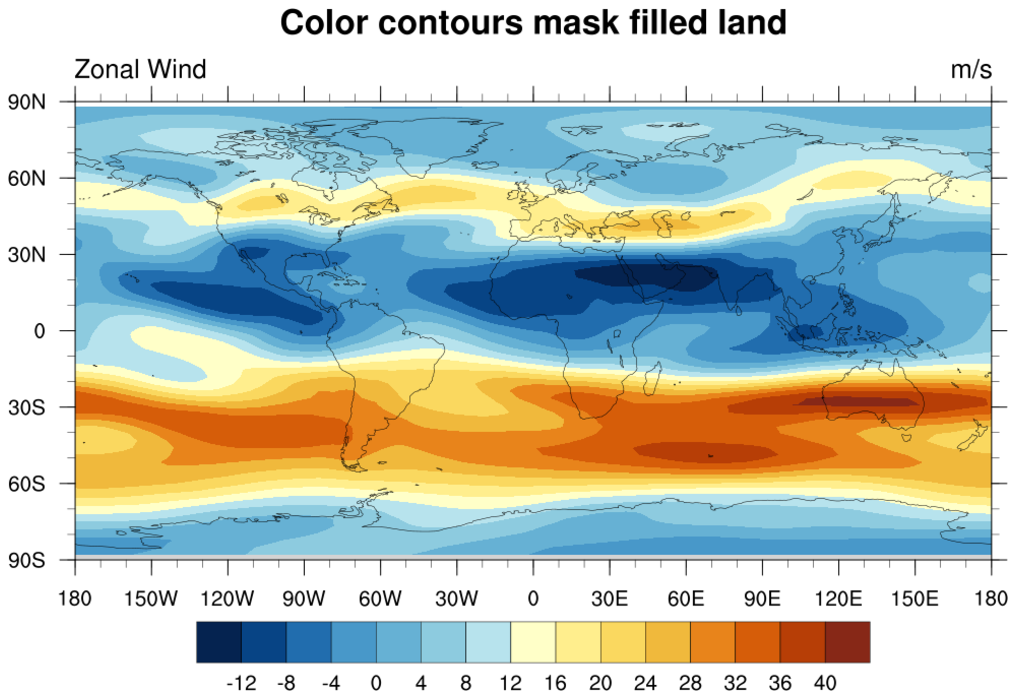
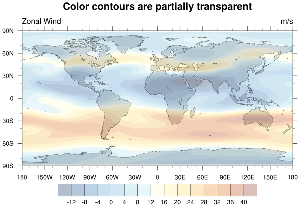
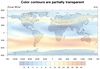 coneff_16.ncl
: Using the
cnFillOpacityF resource to
make the contour fill more transparent. The first frame has
no transparency, and the second frame has some transparency.
You may notice that the filled contours are slightly different over
land. This is because the land is filled in gray.
A Python version of this projection is available
here.
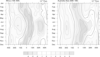
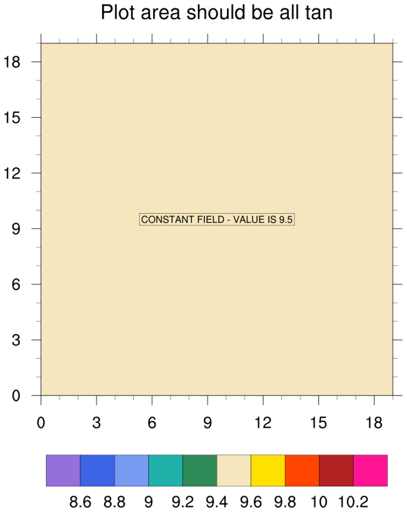
 coneff_17.ncl
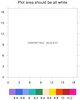
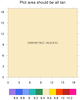
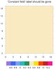
: This example shows
how to force a color fill for a contour field that is constant, by
setting
cnConstFEnableFill to
True. (
This resource may default to this value in a future version
of NCL.)
The first frame shows the default behavior for contouring a constant
field, and the second frame shows the use
of cnConstFEnableFill. The third
frame shows how to turn off the "constant field" label in the middle
of the plot.
There are many resources for customizing the "constant field" label.
Go to the contour resources page
and search for resources starting with "cnConstF".
Note: this script will produce the following warnings:
  warning:ContourPlotInitialize: scalar field is constant; no contour
            lines will appear; use cnConstFEnableFill to enable fill
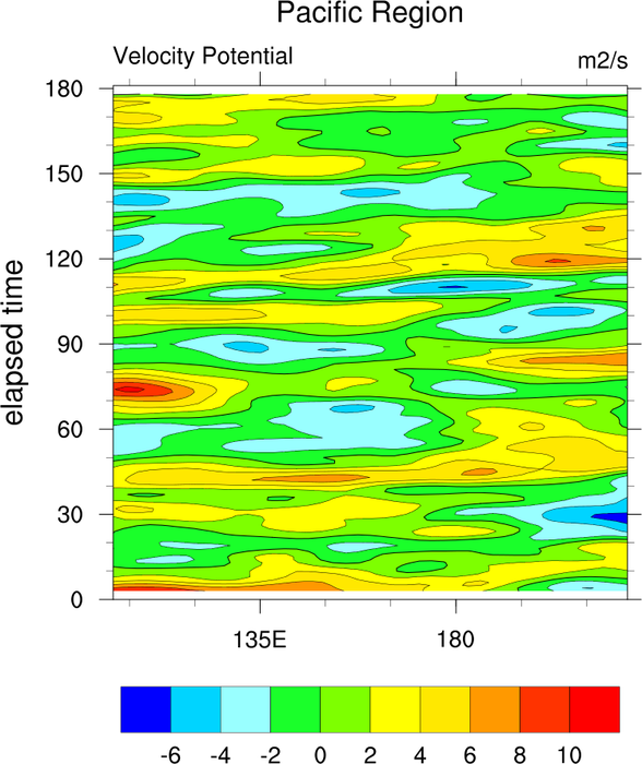
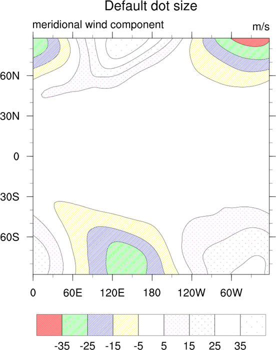
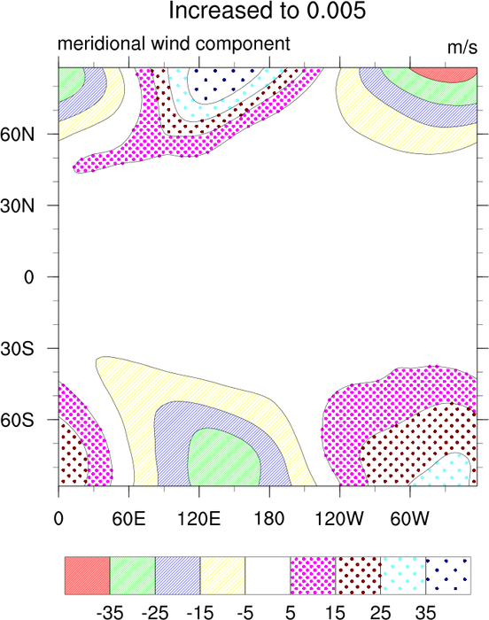
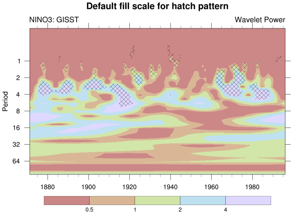
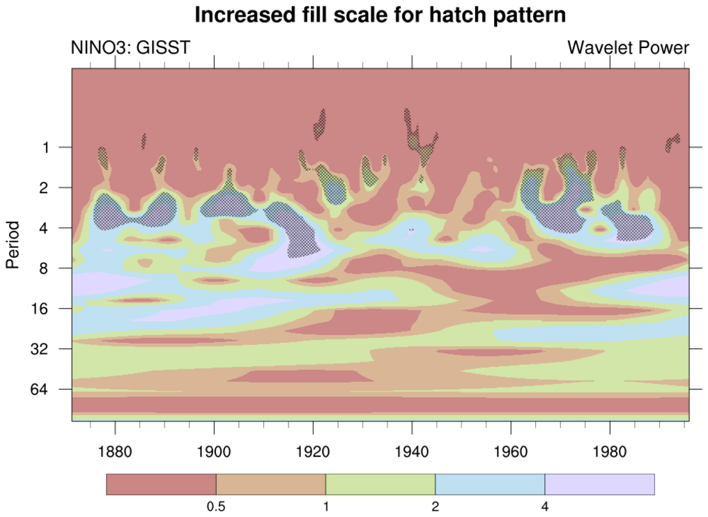
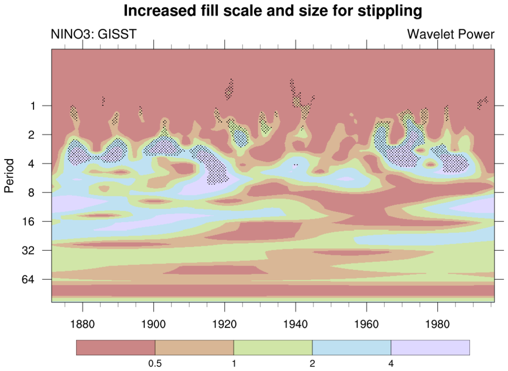
 wavelet_3.ncl
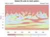
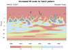
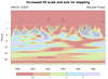
: This example
shows how to use the gsnShadeFillScaleF and gsnShadeDotSizeF
resources to control the density and size of pattern and stipple
shading patterns added by
gsn_contour_shade.
Available in version 6.4.1 and later.
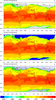
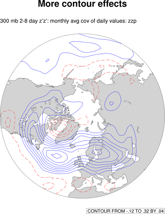
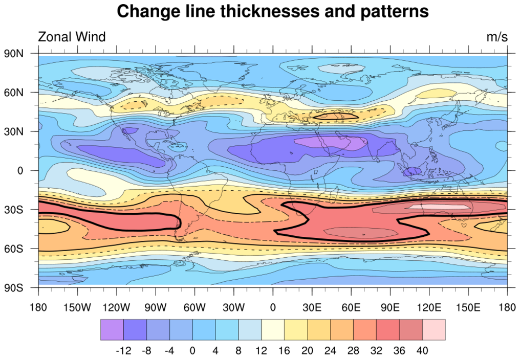
 coneff_18.ncl
: This example shows
how to draw a basic contour map plot, and then modify it by setting
the thickness and dash pattern of the contour lines. This is similar
to the
coneff_4.ncl example, but
shows how to change the thickness of any contour line, not just the
zero line like with
gsnContourZeroLineThicknessF.
You can also use the cnFillOpacity resource
to set the opacity of the contours on a contour plot. It is used in this plot to
emphasize the changes to the contour lines. In addition, this script contains
custom functions to set the patterns and thicknesses of the contour lines based on
either user-specified values or default values.


