NCL Home> Application examples> Plot techniques || Data files for some examples

Example pages containing: tidbits | resources | functions/procedures

Color Fill

List of available color tables.

To reverse a color table, see example 6 on the label bar page.

To add a color (gray) to a colormap, see example 2

gsn_define_colormap is the primary mean of specifying a colormap. This function will accept a built-in NCL named colormap (example 7 and example 2), an array of named colors (example 4), and an array of rgb triplets (example 12). The 650 valid named colors and the corresponding RGB triplets are listed in "$NCARG_ROOT/lib/ncarg/database/rgb.txt."

There's also a separate page for dealing with color maps.

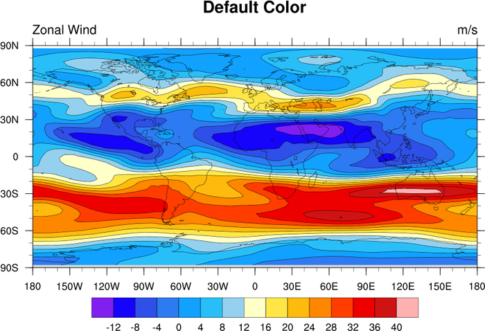
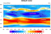color_1.ncl: Demonstrates turning on color with the default color map.

cnFillOn = True, turns on the color fill.

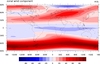
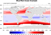color_2.ncl: Example of using a built in colormap. Also demonstrates adding gray to a colormap for the continents if needed.

gsn_define_colormap is the procedure used to set a colormap for the given workstation. There are numerous color tables to choose from.
Setting gsnSpreadColors=True will use all the colors in a color map when creating a filled contour or vector plot. The default is to start with the first color and use them in sequence.

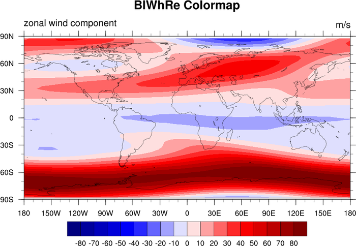
For best results when using the blue/red color spectrum, manually set the contour levels so that the change centers on zero:
cnLevelSelectionMode = "ManualLevels"
cnMinLevelValF
cnMaxLevelValF
cnLevelSpacingF

When you choose a colormap that does not have gray in it, you have to add that color if you want the continental fill to be gray.
i = NhlNewColor(wks,0.8,0.8,0.8) will add the gray.

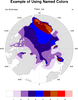color_3.ncl: Demonstrates how to select just a few colors out of a large colormap and make one of those colors transparent.

cnFillColors is the resource used to select what colors out of a colormap you want to represent each contour in the plot.

The -1 indicates that the color is transparent. This is not a true color per say but rather the absence of color. As such, whatever color the background is will be seen.

color_4.ncl: Demonstrates the selection of a color map through individual named colors.

gsn_define_colormap will create a colormap from named colors:
colors = (/"RoyalBlue","LightSkyBlue","PowderBlue"/).

gsn_csm_contour_map_polar is the plot template that draws contours over a polar stereographic map.

gsnPolar = "NH", Selects the hemisphere to plot.

mpMinLatF = 45, Sets the radial extent of a polar plot. In the southern hemisphere, mpMaxLatF should be used.

color_5.ncl: Creates a panel plot with its own label bar.

gsnPanelLabelBar = True
Note that this resource should be passed only to gsn_panel.

You can see other examples of panel plots and common label bars on the special topics panel page.

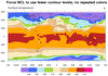
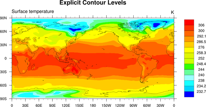
color_6.ncl: Creates a color plot with uneven color intervals.

cnLinesOn = False, turns off contour lines.

cnLevelSelectionMode="ExplicitLevels", and cnLevels = (/232.7,234.2,238,240,244,248.4,252,258.3,276,286.5, 292.1,300,306/) manually sets the uneven contour levels.

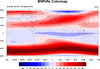
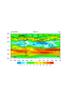
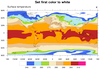
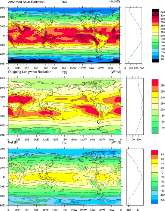
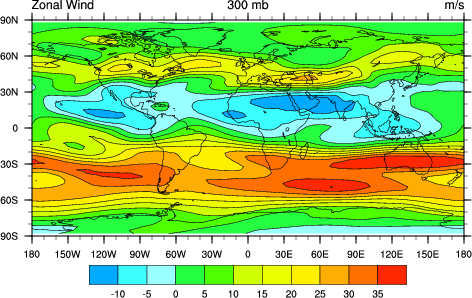
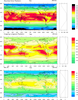color_7.ncl: Another example of choosing from a set of predefined color maps. Zonal average automatically calculated and plotted. The label bar is moved from the default horizontal to vertical.

gsn_define_colormap(wks,"uniform"), Selects the "uniform" predefined color map. There are numerous color tables to choose from.

lbOrientation = "Vertical", Creates a vertical label bar.

gsnZonalMean = True, Automatically calculates and draws the zonal mean of the field. gsnZonalMeanXMaxF and gsnZonalMeanXMinF allow the user to change the axis of the zonal average plot.

color_8.ncl: Draws the colormap. This is useful for debugging or color selection purposes. Also demonstrates how to reverse a colormap.

gsn_draw_colormap and gsn_reverse_colormap draws the colormap and reverse a colormap respectively.

color_9.ncl: Merges two colormaps so that in essence multiple colormaps can be used on the same workstation.

gsn_merge_colormaps merges two colormaps.

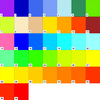
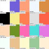
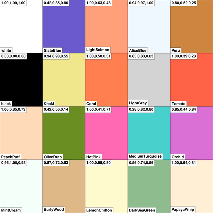
color_10.ncl: I randomly chose colors from the master list of named colors, and placed them in my own RGB file (test_rgb.txt) to create a personalized colormap.

RGBtoCmap is the function that will take a text file of RGB triplets and convert them into an NCL colormap. You can then use gsn_draw_colormap to preview what your colormap looks like. This is an easy way to develop your own colormaps.

color_11.ncl: The American Geophysical Union (AGU) is now requiring all figures submitted for publication to be in CMYK color. This is easily done in NCL.

 type  = "ps"  
 type@wkColorModel = "cmyk"

wks = gsn_open_wks(type,"color"), pass the variable to the workstation routine.

This example, along with many others throughout this web site use three resources to specify how a color table is used. gsnSpreadColors will ensure that the full range of the colormap is used. Otherwise, NCL will take each color in turn and you may end up with an all blue plot for instance if you used a blue_red color table.

gsnSpreadColorStart allows you to choose which color to start your color table at while gsnSpreadColorEnd allows you to choose which color to end your color table.

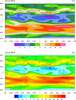
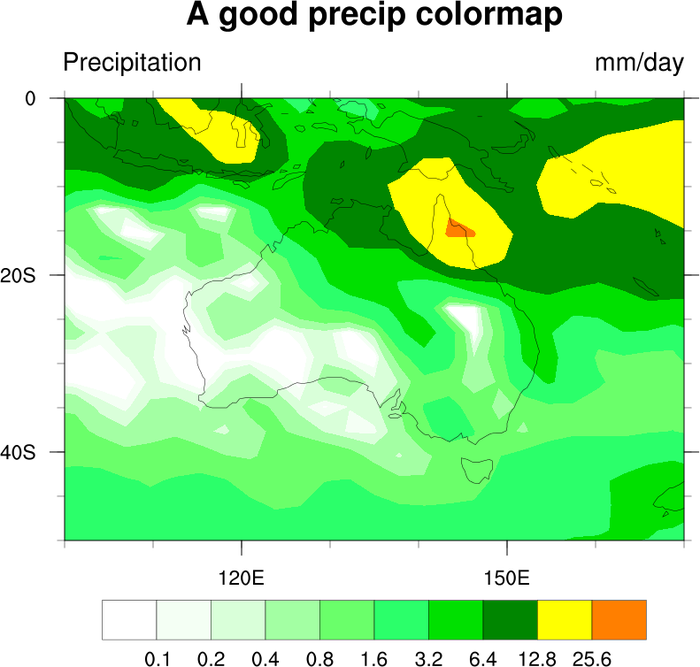
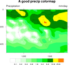color_12.ncl: Demonstrates choosing a colormap based upon the specification of an array of RGB triplets.

The array must be a float array, and must be normalized by dividing by 255.

This particular color map is specifically used for precipitation plots.

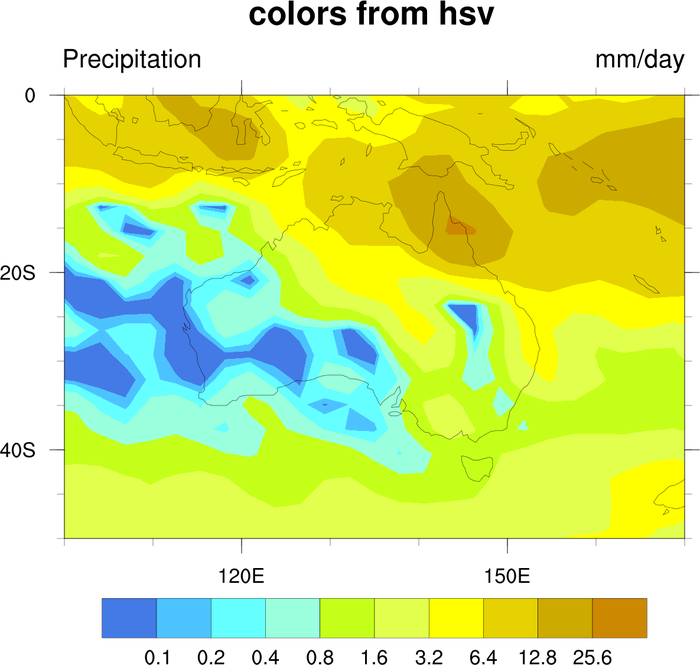
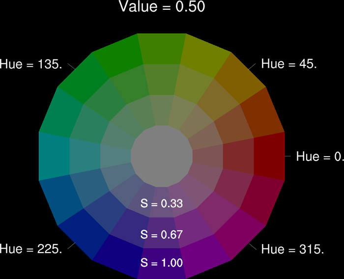
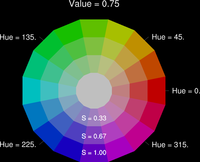
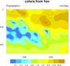color_13.ncl: Demonstrates how to convert an array of colors in HSV format to RGB format.

hsvrgb is the function that does the conversion. See the script for usage. hsvrgb, available in version 4.3.2 or later, replaces the obsolete function hsv2rgb.

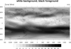
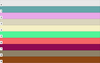
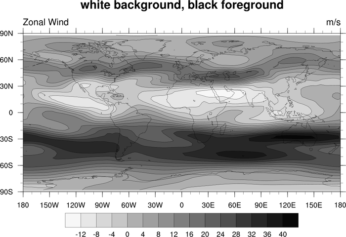
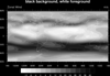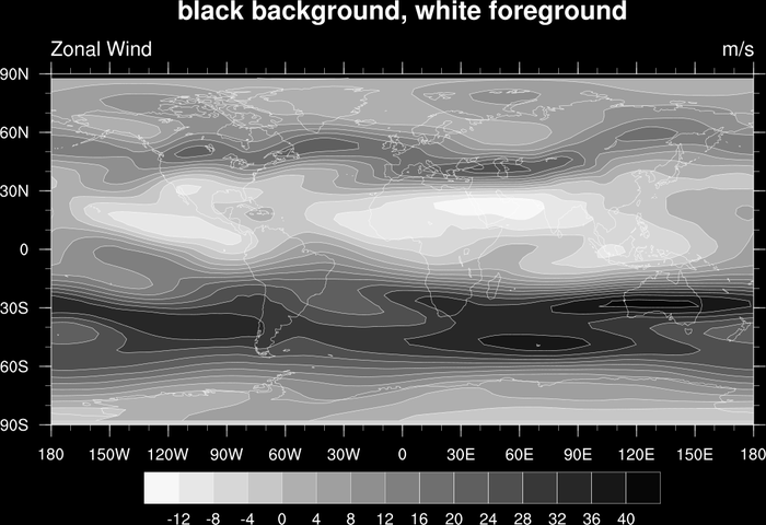
color_14.ncl: Demonstrates what the color table gsltod looks like and how to switch the first two colors. Note that in order to change the foreground and background colors, you must use the wkForegroundColor and wkBackgroundColor resources.

 setvalues wks
   "wkColorMap": "gsltod"  
   "wkForegroundColor" : (/0.,0.,0./)  
   "wkBackgroundColor" : (/1.,1.,1./) 
 end setvalues

will reset the first two colors.

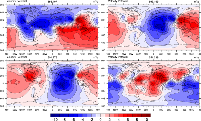
color_15.ncl: Uses symMinMaxPlt to automatically calculate symmetric min/max/int values for use with a symmetric colormap. This is useful when running a script that plots multiple variables of varying magnitudes.

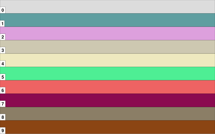
color_16.ncl: Uses gsn_retrieve_colormap to retrieve a colormap and changes one of the colors.

An alternative to this method is to use the function NhlNewColor, which can be used to add a color to the existing colormap, if that colormap has less than 255 colors. 255 is the maximum number of defined colors in a colormap in NCL.

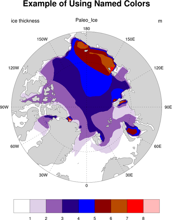
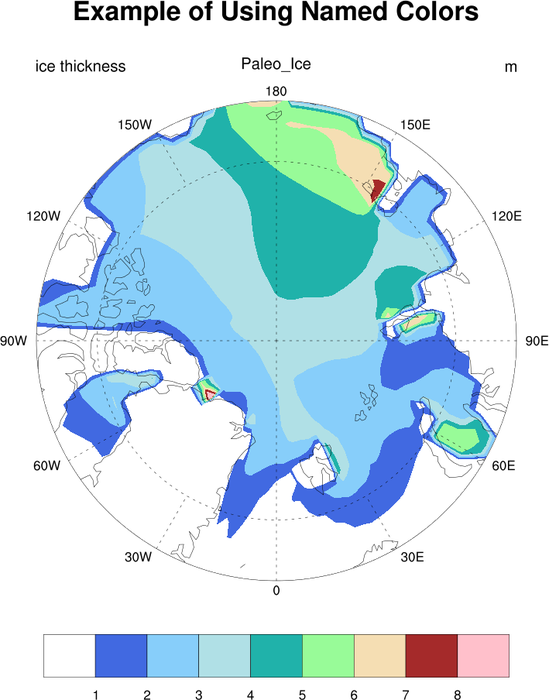
color_17.ncl: Draws the given list of named colors using gsn_draw_named_colors. This is useful for debugging purposes.

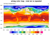
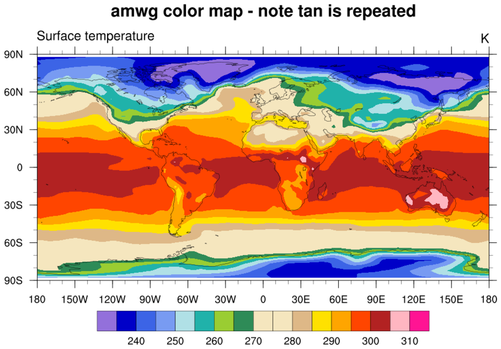
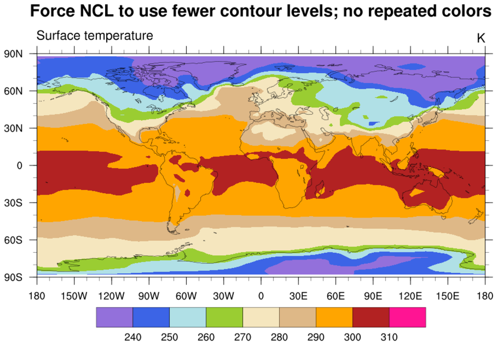
color_18.ncl: Uses hsvrgb to draw some illustrative HSV color wheels. hsvrgb, available in version 4.3.2 and later, replaces the obsolete function hsv2rgb.