WRF

Lambert Conformal Projection

This suite of examples uses an older and deprecated method of plotting WRF data. We recommend that you visit the more up-to-date WRF-ARW Online Tutorial for examples of using NCL to plot WRF-ARW data.

The WRF variables on the 'real data' netCDF file used in the examples are on a native Lambert Conformal projection. By default, when data are placed onto a map, NCL performs a transformation to the specified projection. This transformation is not needed for native grids. To turn off this default behavior, set tfDoNDCOverlay = True. This will result in faster graphic generation.

The gsm_csm_*map* suite of interfaces expect global data. If plotting regionl data, it is necessary to set gsnAddCyclic = False

The WRF netCDF file contains the information needed to properly plot the grid, specifically: (i) the global attributes TRUELAT1, TRUELAT2 and CEN_LON and (ii) the grid latitudes (XLAT) and longitudes (XLONG). The required approach to plotting the data upon a native projection is to specify mpLimitMode = "Corners".

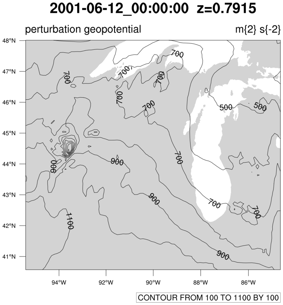
WRF_lc_1.ncl: Basic black and white contour on Lambert Conformal Map. This example explicitly sets all the resources for correctly contouring the data upon a native Lambert Conformal projection. Because the spatial coordinate variables XLAT, XLONG and ZNU do not change with time, only values from the initial time are read.

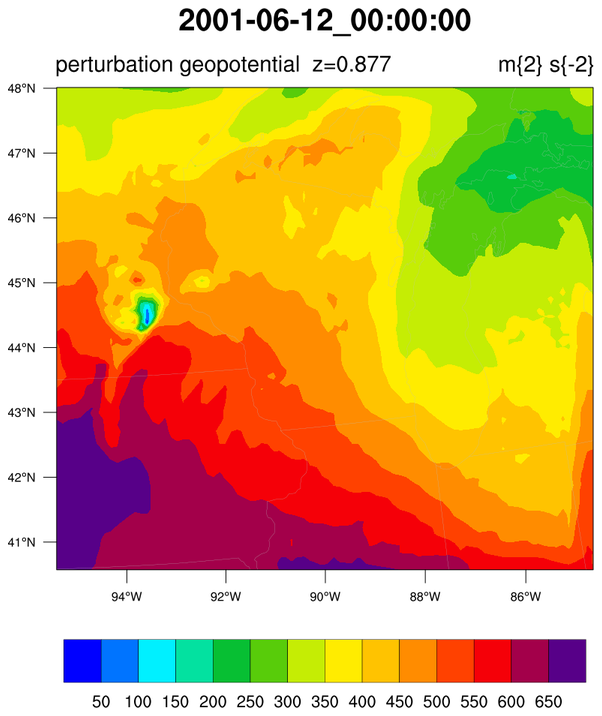
WRF_lc_2.ncl: A color version.

cnFillOn = True, turns on color contours while gsn_define_colormap allows the user to change the color map. This can be from a set of available color tables or various other techniques such as specifying named colors or RGB triplets.

pmTickMarkDisplayMode = "Always" turns on the map tickmarks. The top and right side lat/lon labels may be turned off by setting tmXTOn = False and tmYROn = False.

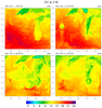
Each native Lambert Conformal Projection plot must specify the same set of map resources. This example, and all subsequent examples on this page, hide these resources in "WRF_map_c" in WRF_contributed.ncl.

WRF_lc_3.ncl: A panel plot.

gsn_panel is the procedure that controls the placement of multiple plots on a page. It expects a different resource variable (e.g. res vs. panel_res) since there are several panel-only options. The panel example page demonstrates these options.

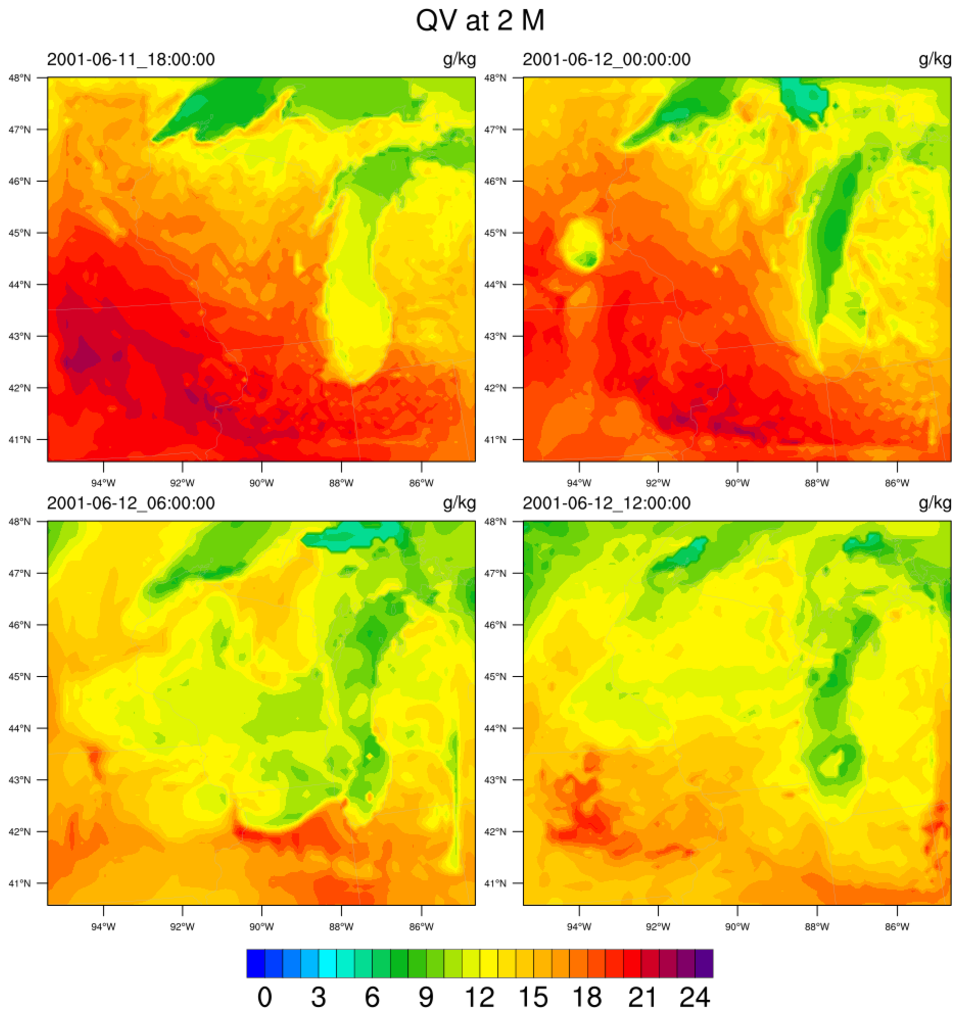
WRF_lc_4.ncl: Panel a specified variable. Plot forecast every 6 hours. When panelling an individual variable, it is desirable to have one common label bar.

nice_mnmxintvl can be used to determine "nice" contour limits.

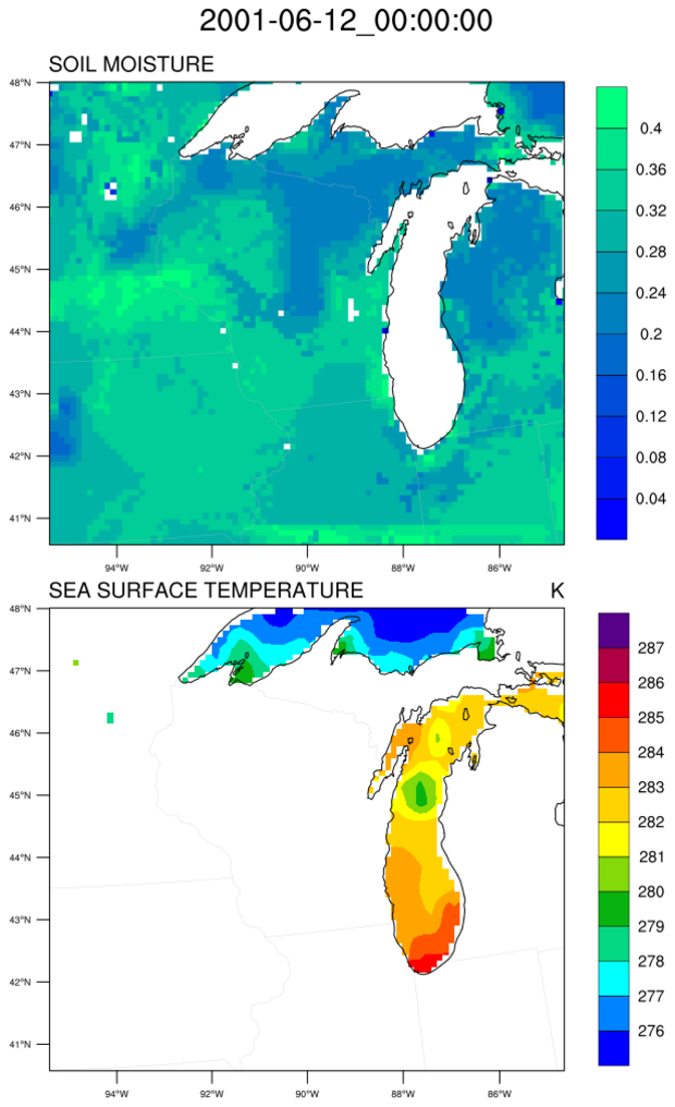
WRF_lc_5.ncl: The WRF netCDF file does not have a missing value attribute (e.g. _FillValue). The SMOIS (soil moisture) and SST (sea surface temperature) variables use 1.0 and 0.0, respectively, to indicate out of range or missing values. These were determined by examining the file. The _FillValue for each variable must be set manually.

The orientation of the label bar can be changed from the default horizontal by setting lbOrientation = "vertical"

cnFillMode = "RasterFill", turns on color rasters.

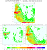WRF_lc_6.ncl: Use the RAINC and RAINNC variables to calculate the total precipitation. Prior to calculating the total, the algebraic operator ">" is used to ensure that negative values are set to zero.

named colors are used create a custom color map. Each color matches the unequally spaced contour levels specified by the user.

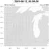
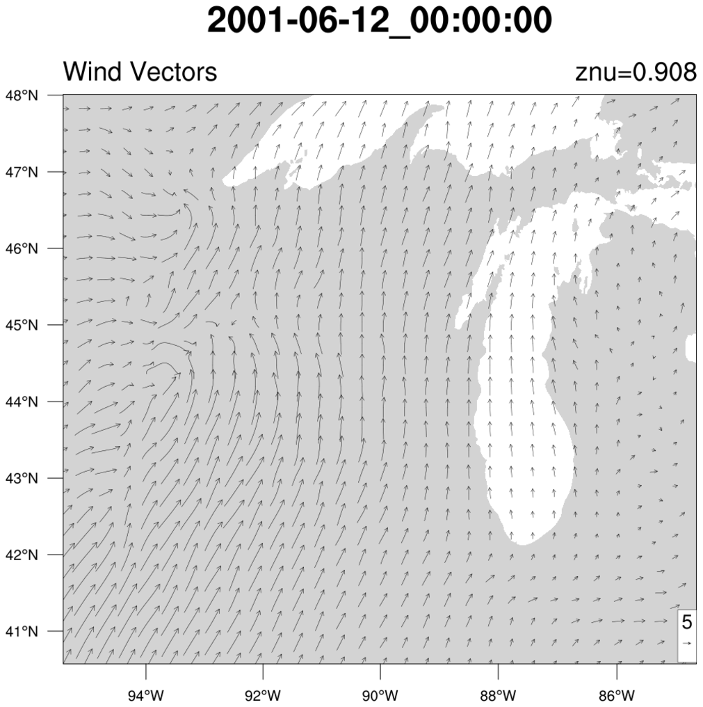
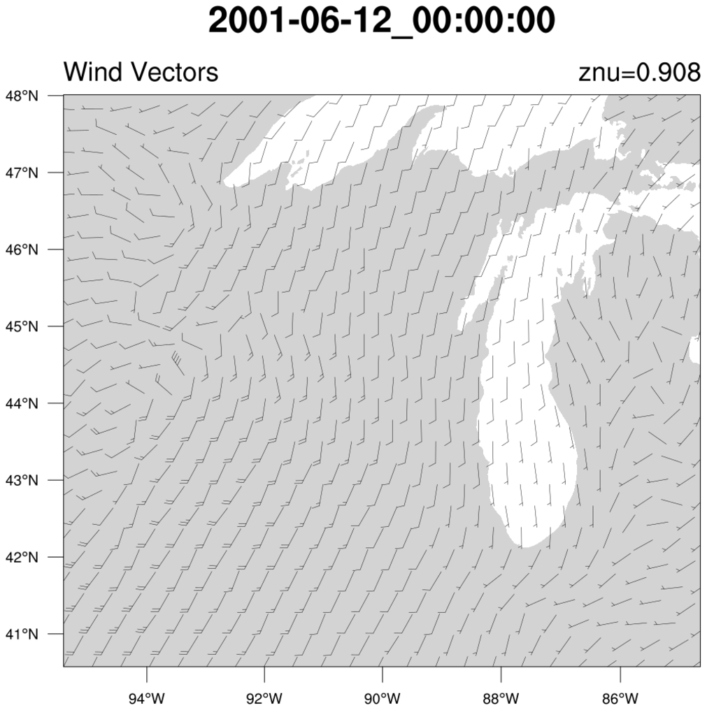
WRF_lc_7.ncl:Basic vectors and wind barbs.

The U and V components are on a staggered grid. Array syntax is used to create u and v on the mass grid whose grid locations are specified by XLAT and XLONG.

u = 0.5*(U(nt,kl,:,0:mlonU-2)+U(nt,kl,:,1:mlonU-1)) 
v = 0.5*(V(nt,kl,0:nlatV-2,:)+V(nt,kl,1:nlatV-1,:))

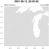
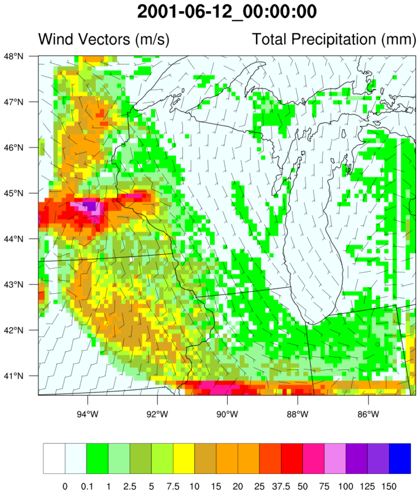
WRF_lc_8.ncl: Overlay winds at 10 meters (U10, V10) over the total precipitation. Meteorological wind barbs are used to indicate direction and speed.

gsnMaximize is used to maximize the image.

WRF_lc_9.ncl: Cross sections along user specified latitudes and longitudes of the Lambert Conformal grid. The eta [ZNU] vertical coordinate is scaled such that it simulates pressure levels. This allows gsn_csm_pres_hgt to be used.